Category Archives: teaching

MEDITES: Parcours Gaia

Pour la troisième année, j’interviens dans le programme MEDITES dans un parcours pédagogique qui présente la recherche en astrophysique à des élèves du secondaire. Cette année, le parcours est focalisé sur les méthodes observationnelles en astronomie: astrométrie, photométrie et spectroscopie, et parlent en particulier de la mission Gaia. Les supports des présentations que j’ai préparés pour l’astrométrie et la photométrie sont disponibles ici.

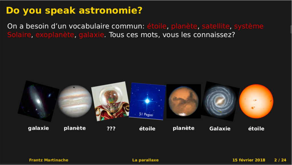
La parallaxe: trouver notre place dans l’univers

Slide extrait d’une présentation sur l’astrométrie et la mesure de la parallaxe faite dans le cadre du programme MEDITES.

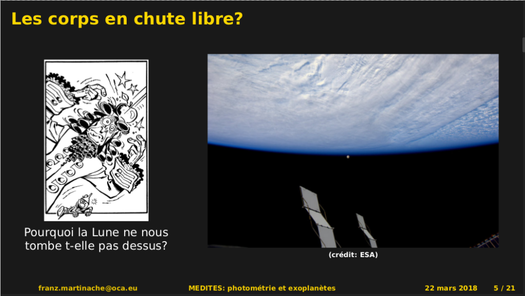
Photométrie et exoplanètes

Slide extrait d’une présentation sur la photométrie et les propriétés physiques des planètes extrasolaires faite dans le cadre du programme MEDITES.

Pour ce parcours, j’ai mis au point et construit une expérience constituée d’un simulateur motorisé de couple étoile-planète et d’une mesure photométrique temps réel par une photodiode connectée à une carte Arduino. J’ai également développé un petit programme d’acquisition des données collectées par la carte Arduino qui permet de faire du traitement a posteriori des données photométriques. Un tutoriel décrivant la fabrication et l’utilisation de cette expérience sera publié cette année par le site du service éducatif de l’Observatoire de la Côte d’Azur.

Parallactic effect while driving

IMPORTANT

Français: Pour que le programme javascript s’exécute correctement, il faut que ce post soit visualisé sans le reste du blog pré-chargé. Si l’image ci-dessous est statique, rechargez le post en cliquant sur son titre ou en suivant ce permalien: merci!

English: For the javascript code to run, this blog post needs to be viewed by itself, ie. without the rest of the blog preloaded. If the image below is not animated, reload the post by clicking on its title or follow this permanent link: thanks!

Wherever I go, the Moon is following me!!

It is an experience surprisingly shared by many: Have you ever felt like the Moon was following you as you drive along a straight road at night? Are we really all that special or is there a simple explanation to this very common perception?

If you carefully look at the following animation, you will notice that, as our character drives along the road, things in the picture do not apparently move at the same speed. Right by the car, the roadside seems to fly by, while the trees, a little further away do seem to move a little slower. The far away mountains also drift, albeit very slowly.

Consider this, the distance that separates the road from the mountains is only of a few dozens of kilometers and they already barely seem to move as one drives by. With this in mind, are you really that surprised that the Moon (400,000 km away) and the stars (light years away) do seem immobile?


Of course, if you wait long enough, because of the Earth’s spin, the postion of the Moon and the stars will begin to drift. But let’s assume that for a few minutes, they don’t. As our character drives along the road, and covers some distance, by looking at how much the mountains have drifted in relation with the “fixed” sky (measuring an angle), he should be able to tell how far the mountain range is from the road.

In astronomy, this principle is used to figure out the distance to the most nearby stars.

The theory of optical stellar interferometry

These videos are part of Section 2 of the on-line course “Eagle Eye Astronomy”, initially released on France Université Numérique. These have recently been re-uploaded on youtube and close-captioned, to help better understand the audio track despite the French accent.

Turn the constraint of diffraction into an advantage: the interferometric trick

Understanding interference fringes: an electromagnetic theory of light

Stars are not lasers: a better model for ordinary light sources

Self-coherence and spatial incoherence of astronomical sources

Transit photométrique

IMPORTANT

Français: Pour que le programme javascript s’exécute correctement, il faut que ce post soit visualisé sans le reste du blog pré-chargé. Si les sliders de la simulation n’ont pas d’effet, rechargez le post en cliquant sur son titre ou en suivant ce permalien: merci!

English: For the javascript code to run, this blog post needs to be viewed by itself, ie. without the rest of the blog preloaded. If the sliders below seem to have no effect on the simulation, reload the post by clicking on its title or follow this permanent link: thanks!

Simulation du transit d’une exoplanète

Cette page propose une simulation numérique du phénomène de transit photométrique d’une planète extrasolaire. Les contrôles de l’expérience, permettent tour à tour de changer:

  • Le diamètre apparent de la planète (en fraction de diamètre de l’étoile). Ex: une valeur de 0.5 veut dire que la planète a un diamètre apparent qui est la moitié de celui de l’étoile.
  • L’inclinaison de l’orbite (en degrés), variant de 0 (système observé par la tranche) à 90 degrés (système vu par les pôles).
  • Le niveau de bruit de la mesure photométrique, exprimé en pourcentage sur la valeur de référence (100%). Une valeur de 0 signifie que les mesures sont parfaites. Le bruit est simulé suivant une distribution gaussienne.

Le cadran de droite permet de visualiser le système: l’étoile, la planète et l’orbite de la planète (circulaire, en blanc) autour de l’étoile. La partie basse affiche la courbe de lumière du système pour les paramètres sélectionnés. Dans le cadran de droite, l’utilisateur peut, en cliquant sur la planète et en la promenant le long de son orbite, relier les différentes parties de la courbe de lumière à la position instantanée de la planète, grâce à la marque jaune superposée à la courbe. Il peut aussi utiliser le slider “position de la planète”.


Contrôles


Mode haute sensibilité


Position de la planète
(degrés)

Diamètre de la planète
(x diamètre étoile)
Inclinaison de l’orbite
(degrés)
Niveau de bruit
(%)


Coherence length

Coherence length and bandwitdh

A finite spectral bandwidth results in some spectral decorrelation of the electric field emanating from a source: even with a true point source, you will only observe the interference phenomenon (mutual coherence of the field) over a finite range of optical path difference (OPD) that is constrained by the coherence length.

Coherence length: Λ0 = λ²/Δλ

An purely monochromatic and phase-calibrated signal like the one coming out of a very good laser would exhibit an infinite coherence length, represented by the green curve plotted below.

Change the bandpass of the filter (here expressed as 1/R=Δλ/λ) to see its effect on the coherence length (the blue curve).

For a given bandpass (say 0.05 and 0.1), how many fringes can you make out in the fringe packet? How do the two quantities (bandpass, number of fringes) relate to each other?


Bandpass

This tool was developed as a part of the on-line course Eagle Eye Astronomy, hosted on the France Université Numérique website.

uv-coverage

Interferometric arrays and spatial frequencies

This post features a pretty fun simulation tool that will allow you to experience “by hand” the relation between the geometry of an interferometric array (that is the location of the telescopes or apertures making up the array) and the corresponding so called “uv-coverage”, that shows all the spatial frequencies the interferometric array gives access to.

The left-hand side plot shows the arangement of apertures. The user can select from several pre-set configurations (Y-shaped, hexagonal-grid, non-redundant) and modify them by moving, adding or removing individual apertures.

Moving one aperture by hand and observing what simultaneously happens on the right-hand side display is particularly “enlightening”: for one, you develop a more intuitive of the relation between one aperture and the different interferometric baselines it is involved with. In addition, you can also observe that geometries laying on a regular grid pattern sometimes result in overlapping points in the uv-plane. The only pattern that strictly avoids this situation is the non-redundant geometry.


?? ??
Resulting uv-coverage

This tool was developed as a part of the on-line course Eagle Eye Astronomy, hosted on the France Université Numérique website.