All posts by Frantz

Kernel-nulling for a robust direct interferometric detection of extrasolar planets

A new paper posted on arxiv by Frantz Martinache & Mike Ireland.

https://arxiv.org/abs/1802.06252

Abstract:

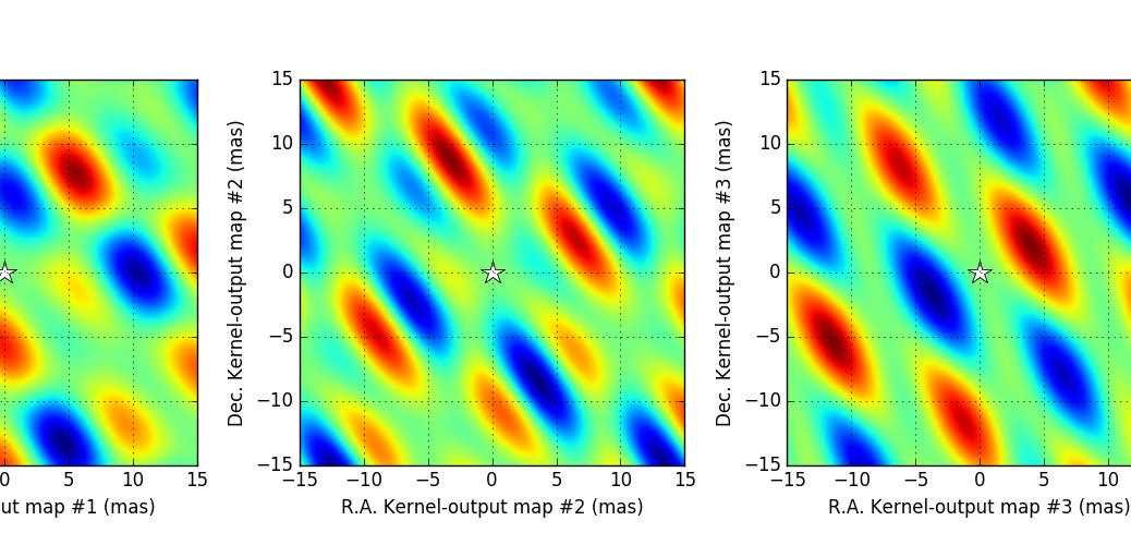
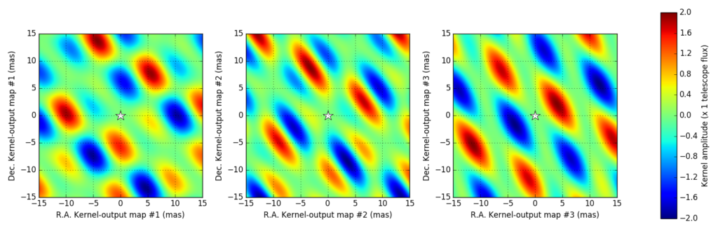
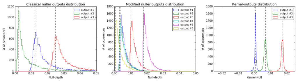
Combining the resolving power of long-baseline interferometry with the high-dynamic range capability of nulling still remains the only technique that can directly sense the presence of structures in the innermost regions of extrasolar planetary systems. Ultimately, the performance of any nuller architecture is constrained by the partial resolution of the on-axis star whose light it attempts to cancel out, and the design of nullers focuses on increasing the order of the extinction to reduce the sensitivity to this effect. However from the ground, the effective performance of nulling is dominated by residual time-varying instrumental phase errors that keep the instrument off the null. This is similar to what happens with high-contrast imaging, and is what we aim to ameliorate. We introduce a modified nuller architecture that enables the extraction of information that is robust against piston excursions. Our method generalizes the concept of kernel, now applied to the outputs of the modified nuller so as to make them robust to second order pupil phase error. We present the general method to determine these kernel-outputs and highlight the benefits of this novel approach. We present the properties of VIKiNG: the VLTI Infrared Kernel NullinG, an instrument concept within the Hi-5 framework for the 4-UT VLTI infrastructure that takes advantage of the proposed architecture, to produce three self-calibrating nulled outputs. Stabilized by a fringe-tracker that would bring piston-excursions down to 50 nm, this instrument would be able to directly detect more than a dozen extrasolar planets so-far detected by radial velocity only, as well as many hot transiting planets and a significant number of very young exoplanets.

December Stromlo KERNEL seminar

Presentation slides of a seminar given at Mt. Stromlo Observatory, in Canberra, Australia.

KERNEL: crack open the walnut
Slide extracted from a presentation introducing the the principles behind kernel-phase and KERNEL project. Click on image to download or access the presentation file!

Parallactic effect while driving

IMPORTANT

Français: Pour que le programme javascript s’exécute correctement, il faut que ce post soit visualisé sans le reste du blog pré-chargé. Si l’image ci-dessous est statique, rechargez le post en cliquant sur son titre ou en suivant ce permalien: merci!

English: For the javascript code to run, this blog post needs to be viewed by itself, ie. without the rest of the blog preloaded. If the image below is not animated, reload the post by clicking on its title or follow this permanent link: thanks!

Wherever I go, the Moon is following me!!

It is an experience surprisingly shared by many: Have you ever felt like the Moon was following you as you drive along a straight road at night? Are we really all that special or is there a simple explanation to this very common perception?

If you carefully look at the following animation, you will notice that, as our character drives along the road, things in the picture do not apparently move at the same speed. Right by the car, the roadside seems to fly by, while the trees, a little further away do seem to move a little slower. The far away mountains also drift, albeit very slowly.

Consider this, the distance that separates the road from the mountains is only of a few dozens of kilometers and they already barely seem to move as one drives by. With this in mind, are you really that surprised that the Moon (400,000 km away) and the stars (light years away) do seem immobile?


Of course, if you wait long enough, because of the Earth’s spin, the postion of the Moon and the stars will begin to drift. But let’s assume that for a few minutes, they don’t. As our character drives along the road, and covers some distance, by looking at how much the mountains have drifted in relation with the “fixed” sky (measuring an angle), he should be able to tell how far the mountain range is from the road.

In astronomy, this principle is used to figure out the distance to the most nearby stars.

Tackling the Low Wind Effect

Because of the exquisite level of wavefront control they enable, extreme adaptive optics (XAO)-fed instruments like SPHERE at VLT or SCExAO at the Subaru Telescope, have led to discovering new subtle effects that were previously invisible, as images were still dominated by the lesser correction. One such recently discovered effect is the “low wind effect” (LWE), so called because its impact is particularly obvious when the low altitude wind speed decreases below a threshold speed: whereas such observing conditions should in theory be ideal for the instrument, the image quality decreases so much that the instrument cannot be used productively.

This effect seems to be due to subtle interactions of the airflow and the structure bearing the secondary mirror of the telescope: when the wind speed drops, temperature gradients occur over the surface of the primary, and result in strong aberrations and even discontinuities in the wavefront that are very difficult to diagnose by conventional wavefront sensors. Given that the signature of the effect is particularly strong on the image (the resulting PSF was even nicknamed “Mickey Mouse”, since it sometimes bears strong sidelobes reminiscent of the famous mouse’s ears), the image seems like the right place to diagnose this effect: an ideal job for the phase transfer model at the heart of the KERNEL project!

Given prior experience with focal plane based wavefront sensing (reported in a publication available here) with the SCExAO instrument, the KERNEL team is investigating the relevance of the asymmetric pupil Fourier wavefront sensing (APF-WFS) technique, and its ability to account for the peculiar aberrations introduced by this LWE. The video below features a proof of concept: it shows that, at least in the context of a simulation, the technique can indeed be used in a closed-loop system, to bring these aberrations down! This adaptation of the APF-WFS to deal with the low wind effect will be the object of experimental work at the Subaru Telescope, over the next couple of weeks.

The theory of optical stellar interferometry

These videos are part of Section 2 of the on-line course “Eagle Eye Astronomy”, initially released on France Université Numérique. These have recently been re-uploaded on youtube and close-captioned, to help better understand the audio track despite the French accent.

Turn the constraint of diffraction into an advantage: the interferometric trick

Understanding interference fringes: an electromagnetic theory of light

Stars are not lasers: a better model for ordinary light sources

Self-coherence and spatial incoherence of astronomical sources

Transit photométrique

IMPORTANT

Français: Pour que le programme javascript s’exécute correctement, il faut que ce post soit visualisé sans le reste du blog pré-chargé. Si les sliders de la simulation n’ont pas d’effet, rechargez le post en cliquant sur son titre ou en suivant ce permalien: merci!

English: For the javascript code to run, this blog post needs to be viewed by itself, ie. without the rest of the blog preloaded. If the sliders below seem to have no effect on the simulation, reload the post by clicking on its title or follow this permanent link: thanks!

Simulation du transit d’une exoplanète

Cette page propose une simulation numérique du phénomène de transit photométrique d’une planète extrasolaire. Les contrôles de l’expérience, permettent tour à tour de changer:

  • Le diamètre apparent de la planète (en fraction de diamètre de l’étoile). Ex: une valeur de 0.5 veut dire que la planète a un diamètre apparent qui est la moitié de celui de l’étoile.
  • L’inclinaison de l’orbite (en degrés), variant de 0 (système observé par la tranche) à 90 degrés (système vu par les pôles).
  • Le niveau de bruit de la mesure photométrique, exprimé en pourcentage sur la valeur de référence (100%). Une valeur de 0 signifie que les mesures sont parfaites. Le bruit est simulé suivant une distribution gaussienne.

Le cadran de droite permet de visualiser le système: l’étoile, la planète et l’orbite de la planète (circulaire, en blanc) autour de l’étoile. La partie basse affiche la courbe de lumière du système pour les paramètres sélectionnés. Dans le cadran de droite, l’utilisateur peut, en cliquant sur la planète et en la promenant le long de son orbite, relier les différentes parties de la courbe de lumière à la position instantanée de la planète, grâce à la marque jaune superposée à la courbe. Il peut aussi utiliser le slider “position de la planète”.


Contrôles


Mode haute sensibilité


Position de la planète
(degrés)

Diamètre de la planète
(x diamètre étoile)
Inclinaison de l’orbite
(degrés)
Niveau de bruit
(%)


Coherence length

Coherence length and bandwitdh

A finite spectral bandwidth results in some spectral decorrelation of the electric field emanating from a source: even with a true point source, you will only observe the interference phenomenon (mutual coherence of the field) over a finite range of optical path difference (OPD) that is constrained by the coherence length.

Coherence length: Λ0 = λ²/Δλ

An purely monochromatic and phase-calibrated signal like the one coming out of a very good laser would exhibit an infinite coherence length, represented by the green curve plotted below.

Change the bandpass of the filter (here expressed as 1/R=Δλ/λ) to see its effect on the coherence length (the blue curve).

For a given bandpass (say 0.05 and 0.1), how many fringes can you make out in the fringe packet? How do the two quantities (bandpass, number of fringes) relate to each other?


Bandpass

This tool was developed as a part of the on-line course Eagle Eye Astronomy, hosted on the France Université Numérique website.

KERNEL pipeline on GitHub!

One of the pillars on which the KERNEL project rests is a data processing pipeline that aims at being as versatile and portable as possible, for general astrophysics purposes as well as for metrology. The maintenance of this tool is one of the tasks listed among the work packages that make up the bulk of the KERNEL project. Since the idea is to make the pipeline available to the community at large, it was decided to host the source code on an open access repository on GitHub. The new package is called XARA, an acronym that stands for eXtreme Angular Resolution Astronomy, and can be downloaded right here. This package is an evolution of a previous incarnation called PYSCO (Python Self-Calibrating Observables), that was hosted on the now defunct Google Code platform. The most notable difference is that it is properly packaged and can be installed, so that its classes and functions can be called from anywhere in your python scripts.

It is accompanied by a convenient simulation package of eXtreme Adaptive Optics (XAO) astutely called XAOSIM and also made available on GitHub. Keep in mind that both are work in progress, that will be regularly updated over the course of the KERNEL project, as features are added and bugs are accounted for, so always check for the latest update of these tools before using them!


uv-coverage

Interferometric arrays and spatial frequencies

This post features a pretty fun simulation tool that will allow you to experience “by hand” the relation between the geometry of an interferometric array (that is the location of the telescopes or apertures making up the array) and the corresponding so called “uv-coverage”, that shows all the spatial frequencies the interferometric array gives access to.

The left-hand side plot shows the arangement of apertures. The user can select from several pre-set configurations (Y-shaped, hexagonal-grid, non-redundant) and modify them by moving, adding or removing individual apertures.

Moving one aperture by hand and observing what simultaneously happens on the right-hand side display is particularly “enlightening”: for one, you develop a more intuitive of the relation between one aperture and the different interferometric baselines it is involved with. In addition, you can also observe that geometries laying on a regular grid pattern sometimes result in overlapping points in the uv-plane. The only pattern that strictly avoids this situation is the non-redundant geometry.


?? ??
Resulting uv-coverage

This tool was developed as a part of the on-line course Eagle Eye Astronomy, hosted on the France Université Numérique website.