XAOSIM templates
Table of Contents
1 High-level API
The fundamental object one manipulates when using XAOSIM for its pseudo real time simulation capability is an instrument. An instrument encapsulates a bunch of other constructs selected among:
- a telescope (class
Telescope) - turbulent phase screens (class
Phscreen) - deformable mirrors (class
DMandHexDM) - cameras (class
Cam,CoroCamandSHCam)
I am sure this creative brain of yours can come up with all kinds of nonsensical combinations of these objects, but the baseline use case is that of a system that features at least one telescope and one camera. At atmospheric phase screen may not be particularly useful for instance if all you want to do is simulate the James Webb Space Telescope.
Telescope here is a big word for what it is in practice in the code: from the point of view of diffractive simulation, the telescope is just a representation of the telescope pupil and a few variables that facilitate its description.
The package comes with a handful of predefined templates for "SCExAO" (of course), "AOC" (a prototype AO system for a 1-meter telescope at Observatoire de la Côte d'Azur), "GRAVITY+" (wrote that one on a dare), "HST" (the NICMOS1 camera) and KERNEL (my current laboratory test bench). My idea is here to show you how you can create your own template from scratch a few of the tools that are part of XAOSIM.
We'll start by creating an empty instrument structure. Let's say we want to create a template for a telescope that we will call "AWESOME". Running the following command:
import xaosim as xs
awesome = xs.instrument("AWESOME", shdir="/dev/shm/", csz=320)
awesome.tel.pdiam = 6.0  # serious telescope upgrade!
will create that structure.
- The first argument is the name of the setup: if the name is one of the default templates (case independant, some loose filtering), then the code will instantiate all of the objects that are part of that setup. Surprisingly, the
AWESOMEsetup does not already exist… so all of the work remains to be done. - The second argument specifies where the shared memory (from now on: SHM) data structures will be created on the Linux system.
/dev/shm/is the default value. If you are running the software on anything but a Linux box, this is probably where you need to adjust: you can decide to create these structures in the current working directory: if that directory is not on a ram mounted disk, read/write access time just won't be as fast but for most simulations, this is probably just fine. - The final argument is an integer:
cszstands for "computation size". This is the size of the arrays that will be used to run Fourier computations. The choice for the exact value is a bit of a tradeoff: small means fast and light, but it has to match the size of the field of view of the camera you want to simulate. For Shack-Hartman simulations, you should make sure that this size is an multiple of the number of cells across one pupil diameter.
By default, awesome features a unobstructed 1-meter diameter circular aperture. I'll defer the description of more realistic pupils when I describe the functions in the pupil module but for now, the above code snippets upgrades bumps the telecope diameter up to 6 meter. We'll simulated an unobstructed 6-meter telescope in space, which would indeed be pretty awesome.
You can already visualze the pupil of the telescope:
import matplotlib.pyplot as plt
plt.imshow(awesome.tel.pupil)
will show the image of a 320x320 array with a circular uniform pupil filling up the array. Careful observation of the edge will show that some effort went into computing a clean transition between what's inside and what's outside the pupil, but more on that later.
2 Camera
Refer to the dedicated page for a more thorough description of the properties and uses of a camera!
By itself, a telescope is not that much fun. Things start getting interesting from the moment you add a camera. Up until now, it's only been useful to have up to two cameras (for instance, one for wavefront sensing and one for imaging): there are two empty references with very creative names (awesome.cam and awesome.cam2) currently set to None waiting to welcome an actual camera reference. Which will be achieved as follows:
awesome.add_imaging_camera(name="cool_cam", ysz=256, xsz=320,
                                                   pscale=10.0, wl=0.8e-6, slot=1)
Adding a camera to an instrument requires a couple of parameters. You can check how instantiating a standalone camera requires additional parameters, but in the context of an instrument, there are already several parameters (such as the computation size, the directory where the shm data structures should be written, …) that have already been decided. This method of the instrument class makes it possible to rely on as few parameters as possible:
nameis a label that describes the camera, here called "cool cam"yszis the "vertical" size of the detector in pixelsxszis the "horizontal" size of the detector in pixelspscaleis the plate scale of the camera (in milli arcsecond per pixel)wlis the central wavelength of observation (in meters)
2.1 Note on the camera plate scale
For this hypothetical example, we have a 6 meter circular aperture feeding a camera with a filtered centered on 0.8 \(\mu m\) (the R band). The formal resolution of one such system is given by the ration \(\lambda/D\), which converted into milliarcsecond gives 200 * 0.8 / 6 ≈ 27 mas. Choosing a plate scale of 10 mas/pixel ensures that the point spread function (PSF) will be sufficiently sampled (∼ 2.7 pixel per resolution element), which is usually a good idea when it comes to interpreting diffraction dominated images. It is of course possible to deliberately undersample if you want by requesting a cruder plate scale, of say 20 mas/pixel, but I have never tried to get anything out of that kind of image so it's up to you.
2.2 Taking images
The thus created camera has the ability to take images of a point source. The following command:
awesome.cam.make_image()
will acquire an image and update the specified SHM structure in /dev/shm/cool_cam.im.shm. To read the content of that image as part of your live python shell, you have to run a separate command that will fetch that image that you can then display with matplotlib:
img = awesome.cam.get_image()
plt.imsave("first_psf.png", img**0.1)
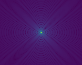
If you had the provided external viewer shmview already displaying the content of the SHM, you may have noticed that the display self-updated from the moment you ran the previous make_image() command.
The Cam class and its specialized versions have a lot of features that it would take too long to describe here. They are further described in a dedicated part of the documentation.
3 Deformable Mirror
Refer to the dedicated page for a more thorough description of the properties and uses of a DM!
Could anything make our already AWESOME unbstructed 6-meter telescope in space more awesome for the pursuit of high contrast imaging? Actually there is, and that would be if the telescope also featured a deformable mirror (DM) that we could use to modulate the shape of the wavefront. Let's just do that and add one such DM: we'll assume that it is a continuous membrane mirror made of a 40x40 grid of actuators. A few of these will lay outside the pupil and won't be useful but we don't have to worry about that with our simulations!
awesome.add_membrane_DM(dms=40, nch=8, na0=39.0, iftype="cosine", ifr0=1.0)
Here is a description of all of the parameters:
instrumentis a human readable label,dmsis the linear DM size in actuator (here 40),nchis the number of channels to create for the DM (see explanation below),shdiris the directory where the camera SHM data structure will be written,shmfis the name of the SHM data structure itself. This also uses the conventional.im.shmextension,na0is the number of actuators that are effectively across one aperture diameter. With a grid of 40x40 actuators, to fully fill the pupil, one will have half an actuator outside of the pupil on all edges and therefore 40-1=39 actuators effectively across the pupil.
This na0 is not automatic because the software can be used to simulate less favorable configurations if needed. There are additional parameters that you can play with that we will revisit in the part of the documentation that is really dedicated to the description of DMs.
With the DM now instantiated, it is now possible to modulate its shape and see the effect of that modulation on the image. For this we need to effectively start the instrument, which will synchronize the state of the camera with that of the DM. Whenever a new command is applied to the DM, the image camera will self update.
awesome.start(delay=0.2)
The delay option is used here to set the pace of the simulation, assuming that your computer has enough CPU to meet this cadence. This semi-real time simulation can be interrupted with:
awesome.stop()
3.1 Virtual DMs, oh my!
Now is the time to talk about this mysterious nch parameter, the number of DM channels created by the simulation. If you've read my intro story of how this software came to be, you know that one of the important features of SCExAO has the ability to multiplex the wavefront control. In practice, this is achieved at the software level by pretending to have an adjustable number of virtual deformable mirrors in the system. An independent program running on the computer constantly monitors the state of these virtual deformable mirror commands (we call these "channels"). Whenever it sees a change occur, it combines the commands present on all the channels into a master command (that in practice include some filtering to avoid sending silly, potentially damaging commands) that is the only one sent to the actual DM electronic driver.
This is such a convenient feature that it is enabled by default in XAOSIM. Here the simulation thus creates 8 separate DM channels that can be addressed separately by external programs or by the current python live shell as we will do here.
3.2 Updating the DM
Assuming that our awesome instrument is running, let us query the channel #0 to get an idea of the required data format to send to the DM, update this with random values (for now) and then send that to the same channel #0. Keep in mind that when operating on an actual instrument that uses the same SHM model to exchange data, the exact same commands sent to the appropriate DM would modulate the real DM!
import numpy as np
dmap = awesome.DM.disp0.get_data()  # returns a 40x40 32-bit float ndarray
dmap1 = 0.01*np.random.randn(40,40) # 40x40 array of random values
awesome.DM.disp0.set_data(dmap1.astype(float32))  # send to channel #0
You can either see the effect of these commands directly using the external shmview live viewer or like before, from your live shell, you have to fetch that image that you can then display with matplotlib:
img = awesome.cam.get_image()
plt.imsave("distorted_psf.png", img**0.1)
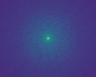
Don't worry too much for now about the box like appearance of the speckle pattern surrounding the PSF at this point. This has to do with the details of the influence function of the deformable mirror which we haven't properly setup yet. We will revisit this in the dedicated DM documentation page.
4 Atmosphere?
Refer to the dedicated page for a more thorough description of the properties and uses of an atmospheric phase screen!
Oh well, I've said that our awesome telescope was in space and didn't have to deal with atmospheric perturbations… but my tour of the template wouldn't be complete without me at least giving you an idea of how to also introduce an atmospheric phase screen… so let's land our telescope somewhere on Earth. Pick your favorite stargazing spot and document yourself about the properties of the atmospheric seeing for that time of the year.
Before adding the atmosphere, it is a good idea to stop the ongoing simulation with a command that was introduced earlier:
awesome.stop()
Adding the atmosphere is very similar to what was done before:
awesome.add_phscreen(name="MaunaKea", r0=0.5, L0=10.0, fc=19.5, correc=1.0)
awesome.atmo.start()
The parameters that are passed along are:
nameis a human readable label,r0is the size of the Fried parameter (in meters),L0is the size of the outer scale parameter (in meters),fcis the AO cutoff frequency expressed in number of cycles across the aperture (don't worry about it now),correcis the uniform AO correction gain over the range of possible spatial frequencies (here again, it will make sense later),
I won't get into a lecture about atmospheric turbulence and will assume that you know what the Fried and the outer scale parameters are. If you don't, then I encourage you to do a little research online. As for the two mysterious fc and correc, their description and the rationale for their existence will be provided in the dedicated section of the documentation. If you start your simulation with the atmosphere now in place, you will observe that things are suddenly a lot more active than what they were before: the atmospheric simulation is self updating rather frequently and a bunch of Fourier computation is now taking place every step of the way to synchronize the camera with the atmosphere. If you use the external viewer, you see the PSF moving in the live display.
4.1 Control the pace!
Depending on your objective and your work conditions, you may not want to try to run this simulation as a fast as your computer allows you to. With the setup we have here, I seem to be able to run the complete simulation at a ∼ 30 Hz pace. Depending on your computer, your version of python (with the 3.8.6 version that I currently use, the CPU usage seems more intense than what I had with 3.6.5), … this can be straining for your computer. The start command takes an optional delay argument which by default is equal to 0.1 second, which means that by default, the simulation refreshes every 0.1 second. You can slow it down further by imposing a longer refresh delay:
awesome.start(delay=0.2)
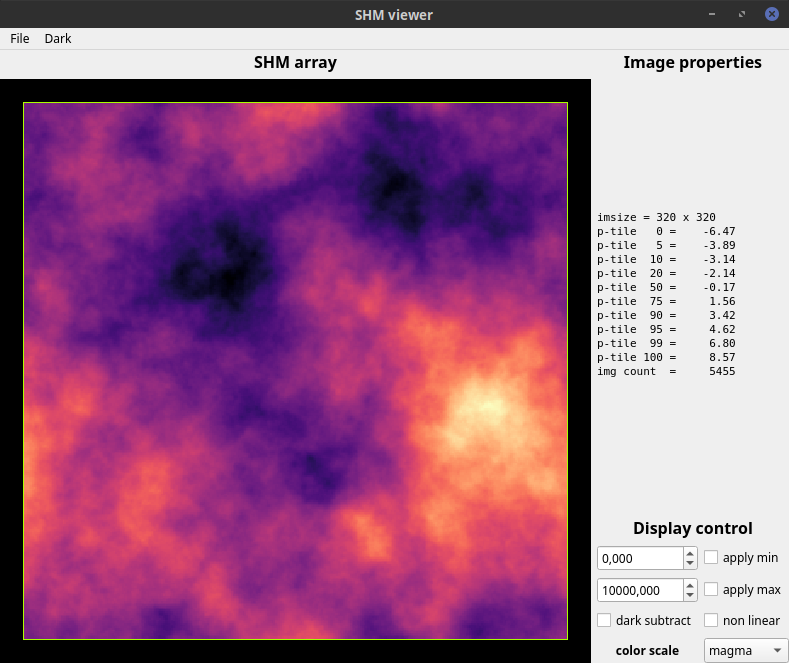
As this is running, you can use the external live viewer to show you what the Kolmogorov phase screen looks like:
5 Complete template
That is a long page for a script that is only effectively 7 lines… but hopefully you now have a better idea of how to do a basic setup for a custom configuration. The complete script, setting up the camera, the DM and the atmosphere and then starting the live simulation is reproduced here to conclude this introduction.
import xaosim as xs

awesome = xs.instrument("AWESOME", shdir='/dev/shm/', csz=320)
awesome.tel.pdiam = 6.0

awesome.add_imaging_camera(name="cool_cam", ysz=256, xsz=320,
  pscale=10.0, wl=0.8e-6, slot=1)

awesome.add_membrane_DM(dms=40, nch=8, na0=39.0,
  iftype="cosine", ifr0=1.0)

awesome.add_phscreen(name="MaunaKea", r0=0.5, L0=10.0, fc=19.5, correc=1.0)

awesome.start(delay=0.2)  # start all servers!