XAOSIM Deformable Mirrors
Table of Contents
1 Introduction
A deformable mirror (DM) is one of the building blocks that make up an instrument cin the context of this simulation package. The fundamental object is defined by the DM class, contained in the DM module of XAOSIM. In this simulation, a DM is always located in the pupil plane and don't plan on integrating DMs at multiple conjugations.
Two types of DMs can be simulated here:
- continuous membrane mirrors deformed by actuators laid out on a square grid
- segmented mirrors made of hexagonal segments that can be controlled in piston, tip and tilt
2 Simulating a membrane deformable mirror
2.1 Basic setup
The instantiation of a DM relies on the following constructor:
import xaosim as xs
mydm = xs.DM(instrument="my instrument", dms=50, nch=8,
                         shm_root="dmdisp", shdir="/dev/shm/",
                         csz=245, na0=49, dx=0.0, dy=0.0,
                         iftype="cosine", ifr0=1.0)
Here is a description of all of the parameters:
nameis a label that describes the instrument, here called "my instrument"dmsis the linear DM size in actuator (here 50),nchis the number of channels to create for the DM (see explanation below),shm_rootis a string that will be used as the root name for the SHM data structuresshdiris the directory where the camera SHM data structure will be written,cszis the computation size: thedms x dmsarray will result in acsz x cszwavefront mapna0is the number of actuators that are effectively across one aperture diameter. With a grid of 50x50 actuators, to fully fill the pupil, one will have half an actuator outside of the pupil on all edges and therefore 50-1=49 actuators effectively across the pupil.dxanddy(in units of actuator size) are alignment offsets between the center of the DM and the center of the pupil.iftypeis a string describing the type of influence function. This is not fully integrated so you can rely on the default for now.ifr0is the influence function radius (in units of actuator size)
By default, the influence function follows the shape of a "cosine" that reaches zero at the distance set by ifr0. Anything other than a "cosine" will result in a sharper "cone" shaped influence function… which turns out to be a reasonably good choice for a lot of simulations in practice.
To be on the safe side of things: just make sure that the csz you choose happens to be an integer multiple of the number of the number of actuators na0 across your pupil.
For now, alignment offsets are a place-holder. These values have no impact on the result of the simulation
2.2 Virtual DMs? Oh my!
Now is the time to talk about this mysterious nch parameter, the number of DM channels created by the simulation. If you've read my intro story of how this software came to be, you know that one of the important features of SCExAO has the ability to multiplex the wavefront control. In practice, this is achieved at the software level by pretending to have an adjustable number of virtual deformable mirrors in the system. An independent program running on the computer constantly monitors the state of these virtual deformable mirror commands (we call these "channels"). Whenever it sees a change occur, it combines the commands present on all the channels into a master command (that in practice include some filtering to avoid sending silly, potentially damaging commands) that is the only one sent to the actual DM electronic driver.
This is such a convenient feature that it is enabled by default in XAOSIM. Here the simulation thus creates 8 separate DM channels that can be addressed separately by external programs or by the current python live shell as we will do here.
To start the channel monitoring process, you have to launch the following command:
mydm.start()
From now on, if something changes on either of the SHM data structures associated to the different channels (assuming that the commands are legit!), the monitor will simply add them and trigger the process that computes a wavefront, using the simulation parameters.
2.3 Interacting with a channel
In this case where we have 8 different channels, references are:
mydm.disp0mydm.disp1mydm.disp2mydm.disp3mydm.disp4mydm.disp5mydm.disp6mydm.disp7
Now if you are a senior programmer with a fair amount of experience in particular in python, you are probably going to want to scream: by the Power of the Grey Skull, why would you do such a thing and why not using a nice data structure like a list or a dictionnary to keep track of the different channels? I hear you, and have been tempted to scream that to the programmer I was eight years ago, when I started putting this code together in python.
The problem is: screams do not travel backward through time. Several high level user applications now expect these variable names to exist and while the idea of setting up aliases to enable some sort of legacy functionnalities has crossed my mind, I haven't been brave enough to implement them yet.
So bear with me for now, even if I eventually change these references. Instead of fixing this, the DM class comes with a handful of higher level functions that allow you to interact with the channels in an easier way:
mydm.set_data_channel(dmap=mydmap, chn=0)sends the command mapmydmapto the channel 0test = mydm.get_data_channel(chn=0)returns the data present on the channel 0mydm.reset_channel(chn=0)resets the command present on the channel 0
A valid command map is a dms x dms 2D ndarray filled with float32 values. Why float32 you ask, since this is no longer the default float size on any self-respecting computer? It is because this software is being used to drive an actual piece of hardware that is expected to run really fast. The resolution of a float64 is not useful (DM drivers have their own DACs that limit the effective resolution of commands being sent to them) and take twice the memory (and therefore slow down the data transfer). We decided early on to stick to float32 values, and have never looked back.
2.4 Membrane DM modulation
2.4.1 Smiley modulation
The following code will show you how to create a valid command, and send it to the DM.
dms = 50
mydmap = np.zeros((dms, dms), dtype=np.float32)
mydmap[24,25] = 1.0  # central actuator
mydmap[12,15:36] = 1.0
mydmap[40,10:20] = 1.0
mydmap[35, 15] = 1.0
mydmap[40,30:40] = 1.0
mydmap[35, 35] = 1.0
mydm.set_data_channel(mydmap, chn=1)
If you haven't started the monitoring process with the mydm.start() command that was covered a few paragraphs ago, you can manually request the system to update once with mydm.update(). Using either of these options, the dms x dms command sent to the channel is combined with whatever is already on the other channels (right now, nothing) and converted into a physical DM displacement map. The simulation places this physical displacement map on a separate SHM data structure (called mydm.wft) that you or another piece of software can read. Let us make a little figure to see the difference between the two:
f1 = plt.figure(figsize=(10,5))
ax1 = f1.add_subplot(1, 2, 1)
ax1.imshow(mydmap)
ax1.set_title("50 x 50 DM command")

ax2 = f1.add_subplot(1, 2, 2)
ax2.imshow(mydm.wft.get_data())
ax2.set_title("Simulated DM displacement")

f1.set_tight_layout(True)
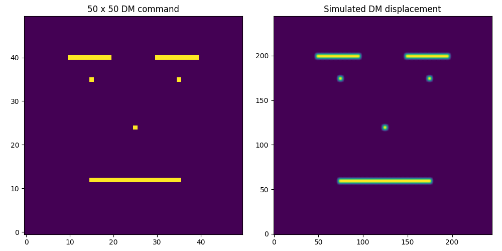
Example of wavefront construction by the DM: side by side comparison of the map of commands and of the wavefront. The result (on the right) is a csz x csz wavefront whose overall structure depends on the influence function.
As cute as the above example can be, this is not a very useful wavefront control command in practice. Luckily, XAOSIM comes with a series of functions to generate useful shapes. Let us look at a couple of examples.
2.4.2 Sinusoidal modulation
The first is that of a 2D sinusoidal modulation, very useful in practice for things like speckle nulling, astrometric grids, … check the documentation of the sin_map function in the wavefront module of XAOSIM for details: here we generate 5 cycles across the horizontal direction and 3 cycles across the vertical.
from xaosim.wavefront import sin_map

cmd1 = sin_map(dms, 5, 3)
mydm.set_data_channel(cmd1, chn=1)
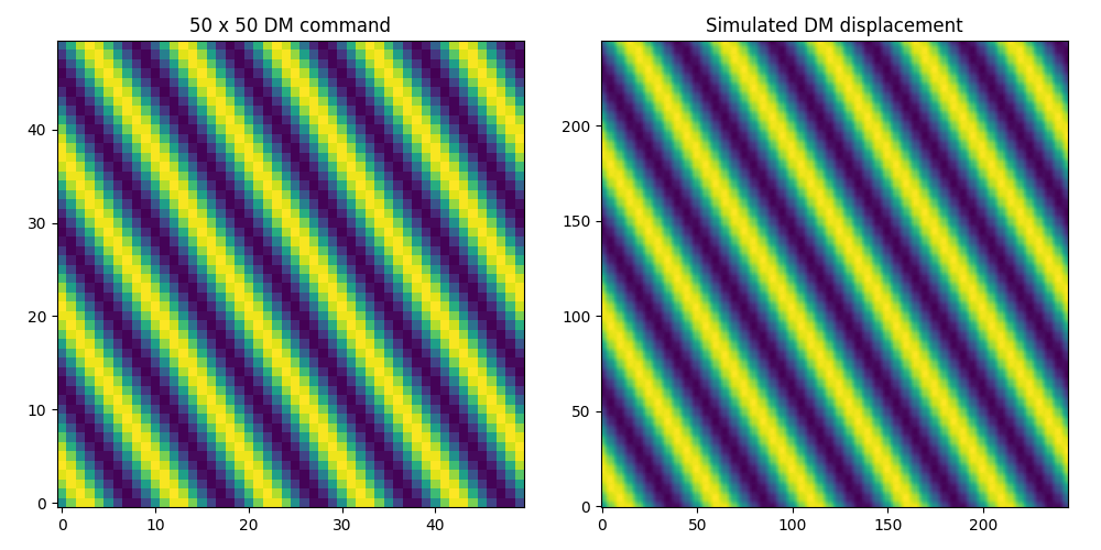
Example of wavefront construction by the DM: side by side comparison of the map of commands and the resulting simulated DM displacement map for a sinusoidal modulation.
2.4.3 Zernike modulation
Another very important class of wavefront shapes is described by the mathematical series known as the Zernike polynomials. Amazingly enough, the first dozen of modes generated by this mathematical series happen to correspond to classical aberrations like focus, astigmatism, coma, … and are therefore widely used in practice. XAOSIM has a dedicated zernike module.
from xaosim.zernike import mkzer1

cmd2 = mkzer1(7, dms, dms//2, True)  # Noll index = 7 -> horizontal coma
mydm.set_data_channel(cmd2, chn=1)
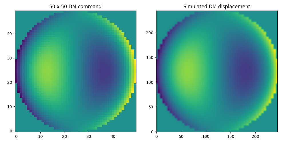 Example of wavefront construction by the DM: side by side comparison of the map of commands and the resulting simulated DM displacement map for horizontal coma.
2.4.4 Crazy modulation
You are of course not limited to sinusoidal and zernike modulations and can load arbitrary shapes, which can be the result of a careful optimisation of modes perfectly adapted to the details of your aperture… or the result of a desperate attempt to scare the speckles away from your field of view… like what is attempted below (the fits file used for this demonstration can be found here). Please be careful when attempting this with an actual deformable mirrors: this kind of modulation might void your warranty.
import astropy.io.fits as pf

cmd3 = pf.getdata("chuck.fits")
mydm.set_data_channel(cmd3, chn=1)
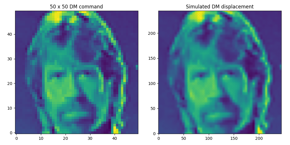 Example of a desperate wavefront control attempt by the DM: side by side comparison of the map of commands and of the DM displacement map effectively generated by the simulation.
2.5 Units and conventions
What units are used for these simulations? Well, when the DM is on its own like we've been using so far, units really do not matter: could be nanometers, meters or radians. Two things to watch out for when the DM is integrated to an instrument with a camera:
- The first one is the
x2effect: Remember that whatever shape you give to your DM gets applied twice to the light that hits the DM (virtue of being a reflective piece of optics). The simulation that computes images for a camera takes that into account and will double the command to estimate the DM-induced wavefront. - The expected units for the wavefront are in microns by default. This default behavior can be altered when updating the properties of an instance of
Cam. The only other option is to express the wavefront in nanometers.
2.6 Influence function
TBD!