XAOSIM Cameras
Table of Contents
1 Introduction
A camera is, along with a deformable mirror and an atmospheric phase screen, one of the building blocks that make up an instrument simulation in the context of xaosim. The basic object is defined by the Cam class, contained in the camera module. A camera is typically the first thing you will want to add to a given instrument. You can refer to the template documentation page to see how to use a camera as part of a complete instrument.
However, assuming that you feed it the right input, a camera can be a self standing object with some useful methods, if you are interested only in static diffractive computation.
2 Diffraction limited imaging
The parameters for a simulation are tied to the physics of diffraction the code is emulating. An instance of camera produces diffracted images relying on Fraunhofer diffraction (also refered to as far field diffraction).
2.1 Sampling of the point spread function
The type of focus of the telescope (primary, Cassegrain, Newton, Coudé, Nasmyth) will change what is refered to as the f-ratio, the ratio between the equivalent focal length for that focus, and the diameter of the telescope: this will in turn, have an effect on the linear size of the theoretical diffraction pattern produced by the telescope given by the product f-number × λ. In practice, how many camera pixels it will take to cover that diffraction pattern depends on the physical size of pixels… which can vary from typically ∼ 1 micron (in the visible) to ∼ 50 microns (in the IR), depending on the technology of detector.
In xaosim, the pitch of the detector and the focus f-ratio are represented by a unique scalar parameter: the instrument plate scale, expressed in milliarcsecond per pixel (mas/pixel). Knowing that plate scale, the diameter of the diffractive aperture (ie the primary mirror of the telescope), and the wavelength at which one observes suffices to contstrain the effective sampling of the camera.
A convenient quick formula can be used to quickly estimate the angular size of the diffraction pattern in milliarcseconds:
\[\alpha \mathrm{(in\, mas)} \approx 200 \times \frac{\lambda \mathrm{(in\, microns)}}{D \mathrm{(in\, meters)}} \]
The number 200 is an approximation of 180 * 3600 / (1000 * π) ≈ 206.265 that converts radians into milliarcseconds.
2.1.1 Examples:
- a 1-meter telescope observing in the visible at wavelength 0.5 microns has a diffraction pattern with a radius of the order of 200 × 0.5 / 1 = 100 mas. If the telescope happens to be perfectly circular and without a central obstruction, that radius will be 1.22 × that previous value.
- a 8-meter telescope observing in the near-IR at wavelength 1.6 microns (in the H-band) has a diffraction pattern with a radius of the order of 200 × 1.6 / 8 = 40 mas.
2.1.2 Sampling
To make sensible observations about the diffraction, the point spread function must be sufficiently sampled, ie. follow the Nyquist-Shannon requirement of at least two pixels per unit of λ/D. This sets an upper limit to the recommended plate scale for your diffractive simulations. Using the examples above, we should specify plate scales no greater than 50 mas/pixel (for the 1-meter telescope observing in the visible) and 20 mas/pixels (for the 8-meter telescope observing in the H-band).
2.2 Diffractive simulations
The overall properties of diffraction dominated images depend on the properties of the diffractive aperture itself and so we must start with something here. If not specified, when creating the instance of camera, the software will simply assume a circular unobstructed aperture. The pupil module of xaosim comes with functions and methods that make it possible to simulate the diffractive aperture of a wide range of real-life telescopes. The aperture will be described by a 2D array of floating point numbers, describing the transmission accross the aperture.
3 Simulating a simple camera
3.1 Initial setup
To only simulate a camera, the following code is required:
import xaosim as xs

mycam = xs.Cam(
        name="cool cam", csz=320, ysz=256, xsz=320,
        pupil=None, pdiam=6.0,
        pscale=10.0, wl=0.8e-6, shdir="/dev/shm/", shmf="cool_cam.im.shm")
Creating a camera on its own requires quite a few parameters… here is a description of the different parameters of the instantiation.
nameis a label that describes the camera, here called "cool cam"cszis the computation size (the size of the Fourier arrays)yszis the "vertical" size of the detector in pixelsxszis the "horizontal" size of the detector in pixelspupilis an array describing the pupil in front of the camera.pdiamis the linear size of the array (in meters) describing the pupilpscaleis the plate scale of the camera (in milli arcsecond per pixel)wlis the central wavelength of observation (in meters)shdiris the directory where the camera SHM data structure will be writtenshmfis the name of the SHM data structure itself. Notice the.im.shmextension that is a convention used to explicitly say that this is a SHM image
It is important to understand the role of the csz parameter: its value will set a limit to the fidelity of the images being computed. As a rule of thumb, you want csz to be equal to the largest dimension of your images. Under the hood, xaosim will actually compute things for square images (of size csz x csz) which will then be cropped down to whatever dimension the user requires (ysz x xsz).
When the value of the pupil parameter is set to None as it is done here, the simulation will use its default setting: an unobstructed circullar telescope.
This created an instance of the Cam class, which is the basic kind of camera that xaosim offers.
3.2 Producing an image
Of course, the really useful thing you can do with a camera is of course, to take a picture. This is how you do it here:
import matplotlib.pyplot as plt

mycam.make_image()      # computes the diffractive image and update the SHM data structure
img = mycam.get_image() # fetches the image
plt.imshow(img**0.2)    # displays the image in a matplotlib window
You can see that bringing an image to your python shell is a two-step process: you first need to compute the image and then, you have to fetch it, for display or further computation. If you use the live display tool shmview that is packaged with xaosim and that monitors in real time, the content of the shared memory data structure, you will see the display change right after calling the mycam.make_image(). Here is what the image gives for the settings listed above:
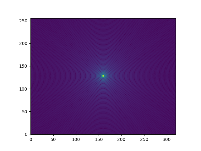 Simulated image of the simulated PSF of a 6-meter circular (unbstructed) aperture at wavelength 0.8 microns with a 320x256 pixel detector and optics that results in a plate scale of 10 mas/pixel
Using the quick formula reminded earlier, for a 6-meter telescope observing at the wavelength 0.8 microns, λ/D ≈ 200 * 0.8 / 6 = 27 mas. With the plate scale of 10 mas/pixel we chose, we have ∼ 2.7 pixel per unit of λ/D and therefore respect the sampling requirement.
3.3 Updating the camera parameters
Given that with a camera on its own, everything is static you will not see that much action… There are still a few intersting way to interact with the simulation that can be informative:
- you can modify the wavelength of observation or the plate scale of your camera using
mycam.update_cam() - you can also add Poisson noise to your image using
mycam.update_signal()
3.3.1 Camera settings
The following code will increase the wavelength from 0.8 to 2.2 microns.
mycam.update_cam(wl=2.2e-6) # filter switch to 2.2 microns
img = mycam.get_image()     # fetches the image
plt.imshow(img**0.2)        # displays the image in a matplotlib window
Without changing the detector plate scale, one expects the PSF get bigger by a factor ~3. The following image will confirm that prediction.
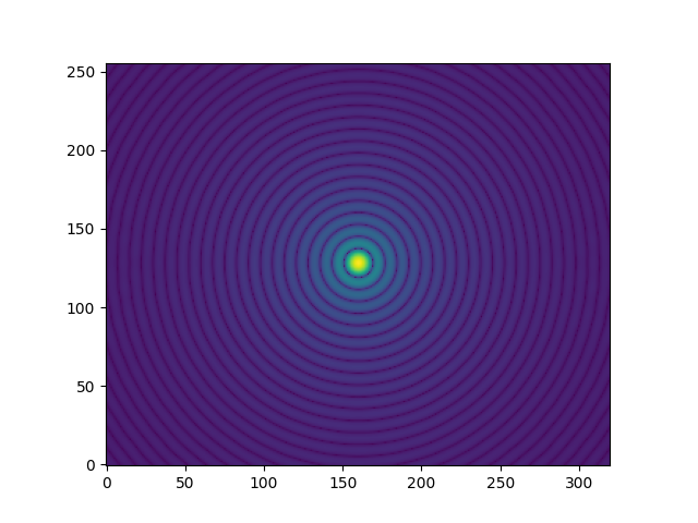 Simulated image of the simulated PSF of a 6-meter circular (unbstructed) aperture at wavelength 2.2 microns with a 320x256 pixel detector and optics that results in a plate scale of 10 mas/pixel
3.3.2 Photon-noise
The images above feature no noise. An important source of noise for diffraction dominated observations (other than speckle noise, which we'll introduce with atmospheric phase screens) is photon-noise, that follows Poisson statistics. The one thing to set up is the total illumination of the detector, ie the total number of photons (assuming a quantum efficiency of 100%) that hits the detector:
mycam.update_signal(1e5) # sets illumination level & photon noise flag to True
img = mycam.get_image()  # fetches the image
plt.imshow(img**0.2)     # displays the image in a matplotlib window
Setting the value with the update_signal() function does two things:
- it changes the level of illumination to the specified total number of photons (here 105 photons)
- it sets the flag
mycam.phot_noisetoTrue
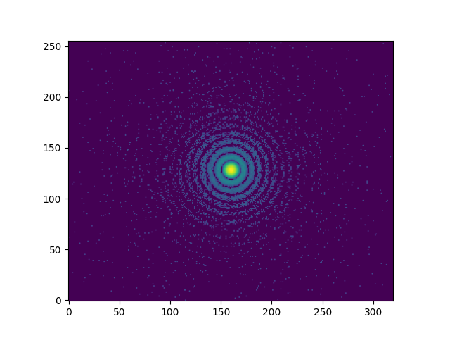 Simulated image of the simulated PSF of a 6-meter circular (unbstructed) aperture at wavelength 2.2 microns with a 320x256 pixel detector and optics that results in a plate scale of 10 mas/pixel. In addition to the diffraction, this simulation also integrates the effect of photon noise, assuming a total illumination of 105 photons over the detector.
To remove the effect of photon noise simply requires to set the flag back to False:
mycam.phot_noise = False
3.4 Updating the pupil
All of the images computed above were for the default unbstructed circular pupil. xaosim features a module that offers the means to compute a wide variety of telescope apertures. The first thing you can do to make sure to get things right, is to visualize the current aperture, which is easy enough:
plt.imshow(mycam.pupil)
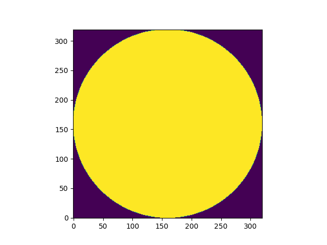 Circular aperture assumed for the Fourier diffractive computation examples above
This array is of size 320x320 (this was set when setting the value of csz at class instantiation). To simulate a new pupil you just need to replace this array with a new array of the same size. I will just produce two examples here and display side by side, the pupil and the ideal diffraction pattern that it results in (still for wavelength of 2.2 $μ$m).
3.4.1 Sparse aperture imaging
sam = xs.pupil.SPHERE_IRDIS_SAM # get the SAM pupil function from the module
mycam.pupil = sam(320) # use that to fit a SAM-like pupil inside the aperture
mycam.make_image()
img = mycam.get_image()

f1 = plt.figure(figsize=(10,5))
ax1 = f1.add_subplot(1, 2, 1)
ax2 = f1.add_subplot(1, 2, 2)
ax1.imshow(mycam.pupil)
ax2.imshow(img**0.2)
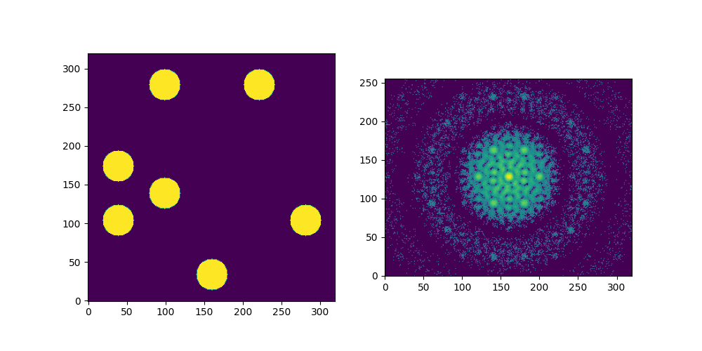 Sparse aperture mask used by SPHERE and the interferogram it results in (photon noise introduced earlier still present.
3.4.2 Subaru telescope aperture
subaru = xs.pupil.subaru            # get the Subaru pupil function from the module
mycam.pupil = subaru(320, 320, 150) # use that to fit a SAM-like pupil inside the aperture
mycam.make_image()
img = mycam.get_image()

f1 = plt.figure(figsize=(10,5))
ax1 = f1.add_subplot(1, 2, 1)
ax2 = f1.add_subplot(1, 2, 2)
ax1.imshow(mycam.pupil)
ax2.imshow(img**0.2)
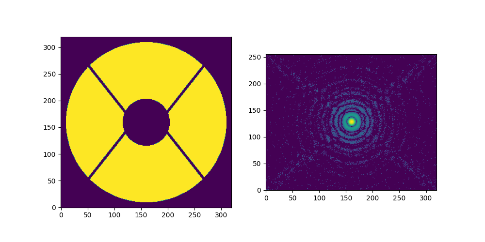 Subaru Telescope pupil and its point spread function (photon noise introduced earlier still present.
3.5 Additional remarks
A glance at the source code will reveal that the Cam class offers additional methods. Some of them are of limiited interest when a camera is created as a standalone object like here and will only become useful when integrating a camera to an instrument. There are two methods that could be discussed here: the sft() method used to do all the Fourier computation and the off_pointing() function that adds an overall phase slope across the pupil. In the context of an imaging camera, this only moves the PSF around. The sft function will probably get its own documentation page (there is even a separate sft module as part of xaosim) so I will not cover it here. The off-axis pointing feature will be covered in the next part of this documentation, describing a special case of a camera that includes the simulation of a coronagraph.
4 Coronagraphic camera
4.1 Initial setup
The CoroCam class inherits from most of the properties of the fundamental Cam class. A lot of the same parameters will have to be set when instantiating a coronagraphic camera. There are however a few additional parameters that require some prior work: the simulation assumes that one can insert:
- a focal plane mask in an intermediate focal plane and
- a Lyot-stop in the exit pupil plane.
If you have no idea what I am talking about here, you probably have no business reading this part of the documentation and should go read some basic papers. I would recommend the proceedings of the 2003 school on "Astronomy with high contrast imaging: from planetary systems to active galactic nuclei" (which I attended as a PhD student) or a more recent paper I wrote after giving a lecture on this topic at the 2017 Evry Schatzman School on "Diffraction-dominated observational astronomy".
This is an example of instantiation of a coronagraphic camera:
import xaosim as xs

mycorocam = xs.CoroCam(
        name="corocam", csz=400, ysz=256, xsz=320,
        pupil=None, fpm=None, lstop=None,
        pdiam=7.92, pscale=16.7, wl=1.6e-6,
        shdir="/dev/shm/", shmf="corocam.im.shm")
Notice that here, pupil, fpm and lstop are all set to None. When nothing is specified here, the simulation falls back onto a default setup:
- an unobstructed circular aperture for the pupil (like we saw in the imaging camera scenario)
- a circular 4 λ/D radius occulting focal plane mask
- a default Lyot-stop that is a 10% undersized version of the input pupil
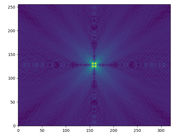
Taking an image with that camera is no different than with the standard:
mycorocam.make_image()
img = mycorocam.get_image()
plt.imshow(img**0.2)
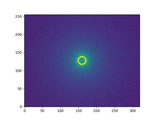
On-axis coronagraphic image for an ideal 4 λ/D radius Lyot-type coronagraph, with a 10% undersized Lyot-stop. The central core of the original PSF is gone and the brightest feature is now a ring that marks the location of the edge of the focal plane.
4.2 Off-axis pointing
All of that is nice already but what else can you do with this camera? The features we've already covered in the case of the imaging camera can still be used (changing the wavelength or the plate scale). The effect will however begin to diverge and no longer just look like a simple overall scaling effect: unless you scale the size of the focal plane mask accordingly, increasing the wavelength will reduce the effective size of the focal plane and reduce the efficiency of the coronagraph. Although I won't do that here, I encourage you to try things out.
What we'll do here however is move the source to the side so as to observe the way the response of the coronagraph changes when a source lands in the vicinity of the focal plane mask. Using the quick formula again, we know that λ/D = 200 * 1.6 / 8 ≈ 40 mas. We can move the target to the side by increments of 20 mas (which is a bit more than one pixel at a time). To make sure the core of the off-axis PSF misses the focal plane mask entirely, we need to move the by at least 4 * 40 = 160 mas. Let's play it very safe and move all the way out to 300 mas to the side, in increments of 20 mas to get a total of 15 images.
For this, we will use the off_pointing() method of the Cam class that the CoroCam inherits. The documentation of that function (accessible from your python shell using: help(mycorocam.off_pointing) reveals that the expected unit for the pointing offsets are in pixels.
step = 20 / mycorocam.pscale
nstep = 15  # number of images
offxs = step * np.arange(nstep)  # array of horizontal offsets
dcube = np.zeros((nstep, mycorocam.ysz, mycorocam.xsz))  # empty datacube
for ii, offx  in enumerate(offxs):
  offset = mycorocam.off_pointing(offx, 0.0)
  mycorocam.make_image(phscreen=offset)
  dcube[ii] = mycorocam.get_image()
dsz = 40
x0, x1 = mycorocam.xsz//2 - dsz, mycorocam.xsz//2 + dsz
y0, y1 = mycorocam.ysz//2 - dsz, mycorocam.ysz//2 + dsz

f1 = plt.figure(figsize=(10, 6))
for ii in range(nstep):
  ax = f1.add_subplot(3,5, ii+1)
  ax.imshow(dcube[ii, y0:y1, x0:x1]**0.2, vmax=8.7)
  ax.set_xticks([])
  ax.set_yticks([])
  msg = "%d mas offset" % (ii * 20)
  ax.text(dsz, 10, msg, ha="center", weight="bold", c="white")

f1.set_tight_layout(True)
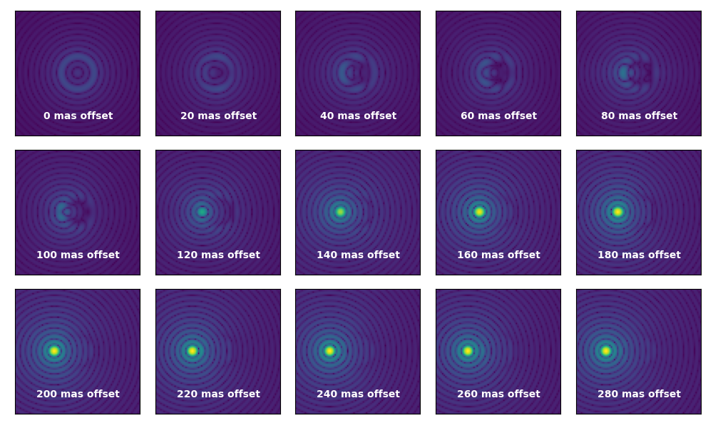 Evolution of the response of the coronagraph as the system is pointed off-axis toward the right (and the targets moves to the left) by 20 mas increments. To observe the evolution of the response and allow comparison between images, the display uses a non-linear scale with a fixed maximum value.
You can convince yourself that the coronagraphic simulation is acting as expected by plotting the evolution of the total flux as a function of the magnitude of the pointing offset:
plt.figure()
step_mas = 20.0 # 20 mas per step
plt.plot(np.arange(nstep) * step_mas, dcube.sum(axis=2).sum(axis=1))
plt.plot(np.arange(nstep) * step_mas, dcube.sum(axis=2).sum(axis=1), 'o')
plt.xlabel("Pointing offset (in mas)")
plt.ylabel("Total flux in coronagraphic image")
plt.title("Off-axis coronagraphic throughput")
plt.tight_layout()
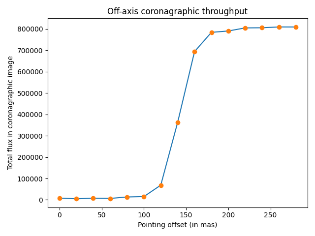
Evolution of the integrated throughput as a function of pointing offset. The 50 % throughtput mark is reached for a separation of ∼ 140 mas: this would set the conventionally accepted value of the coronagraphic inner working angle (IWA).
The inner working angle (IWA) of a coronagraph is conventionnally defined as the angular distance beyond which the off-axis throughput approaches 50 %. According to the above plot, the IWA for this setup would be 140 mas.
4.3 What about my favorite coronagraph?
To set up your favorite coronagraph, you simply need to update the focal plane mask and the Lyot stop with arrays of the appropriate size csz. There is at the moment no high-level API to update these components and you have to directly replace the existing properties of mycorocam in place. The following code shows you how to update the focal plane mask with a four quadrant phase mask:
from xaosim.pupil import fqpm

mycorocam.fpm = fqpm(mycorocam.csz)
mycorocam.make_image()
img = mycorocam.get_image()
plt.imshow(img**0.2)
On-axis coronagraphic image for an ideal four quadrant phase mask coronagraph, with the same 10% undersized Lyot-stop that was used previously.
4.4 Under the hood!
If speed is paramount for your simulation, the different steps of the coronoagraphic simulation should be integrated into a single linear operation acting on the input electric field to produce an intensity map of the post-coronagraphic electric field. Because XAOSIM is also a teaching tool, the simulation gives access to the intermediate optical planes so as to reveal what each part of a coronagraph does to the electric field. I will do just that for the Lyot-coronagraph we started with.
The class attributes have "hidden" names, starting with the underscore character. The following table gives you the key for these otherwise hard to guess names!
| Class member name | Description |
|---|---|
mycorocam._b4m |
Complex amplitude before (b4) the focal plane mask |
mycorocam._afm |
Complex amplitude after the focal plane mask |
mycorocam._b4l |
Complex amplitude before the lyot-stop |
mycorocam._afl |
Complex amplitude after the Lyot-stop |
mycorocam._cca |
Complex amplitude in the coronagraphic focal plane |
The following code snippet produces a nice figure that shows the modulus of the complex amplitude in these different planes for a source on-axis and for a source off-axis. The simulation part only takes two make_image() commands: the bulk of this code is to make a nice figure with matplotlib, which sometimes takes some effort.
dsz = 40
csz = mycorocam.csz
x0, x1 = csz//2 - dsz, csz//2 + dsz
y0, y1 = csz//2 - dsz, csz//2 + dsz

f1 = plt.figure(figsize=(15, 6))
f1.set_tight_layout(True)

mycorocam.make_image()

ax = f1.add_subplot(2, 5, 1)
ax.imshow(np.abs(mycorocam._b4m)[y0:y1, x0:x1]**0.4, vmax=8.7)
ax.tick_params(left=False, bottom=False, labelleft=False, labelbottom=False)
ax.text(dsz, 10, "original PSF", ha="center", weight="bold", c="white")

ax = f1.add_subplot(2, 5, 2)
ax.imshow(np.abs(mycorocam._afm)[y0:y1, x0:x1]**0.4, vmax=8.7)
ax.tick_params(left=False, bottom=False, labelleft=False, labelbottom=False)
ax.text(dsz, 10, "focal plane mask", ha="center", weight="bold", c="white")

ax = f1.add_subplot(2, 5, 3)
ax.imshow(np.abs(mycorocam._b4l))
ax.tick_params(left=False, bottom=False, labelleft=False, labelbottom=False)
ax.text(csz//2, 0.125*csz, "pupil before Lyot-stop", ha="center", weight="bold", c="white")

ax = f1.add_subplot(2, 5, 4)
ax.imshow(np.abs(mycorocam._afl))
ax.tick_params(left=False, bottom=False, labelleft=False, labelbottom=False)
ax.text(csz//2, 0.125*csz, "pupil after Lyot-stop", ha="center", weight="bold", c="white")

ax = f1.add_subplot(2, 5, 5)
ax.imshow(np.abs(mycorocam._cca)[y0:y1, x0:x1]**0.4, vmax=8.7)
ax.tick_params(left=False, bottom=False, labelleft=False, labelbottom=False)
ax.text(dsz, 10, "coronagraphic PSF", ha="center", weight="bold", c="white")

offset = mycorocam.off_pointing(15, 0)
mycorocam.make_image(phscreen=offset)

ax = f1.add_subplot(2, 5, 6)
ax.imshow(np.abs(mycorocam._b4m)[y0:y1, x0:x1]**0.4, vmax=8.7)
ax.tick_params(left=False, bottom=False, labelleft=False, labelbottom=False)
ax.text(dsz, 10, "original PSF", ha="center", weight="bold", c="white")

ax = f1.add_subplot(2, 5, 7)
ax.imshow(np.abs(mycorocam._afm)[y0:y1, x0:x1]**0.4, vmax=8.7)
ax.tick_params(left=False, bottom=False, labelleft=False, labelbottom=False)
ax.text(dsz, 10, "focal plane mask", ha="center", weight="bold", c="white")

ax = f1.add_subplot(2, 5, 8)
ax.imshow(np.abs(mycorocam._b4l))
ax.tick_params(left=False, bottom=False, labelleft=False, labelbottom=False)
ax.text(csz//2, 0.125*csz, "pupil before Lyot-stop", ha="center", weight="bold", c="white")

ax = f1.add_subplot(2, 5, 9)
ax.imshow(np.abs(mycorocam._afl))
ax.tick_params(left=False, bottom=False, labelleft=False, labelbottom=False)
ax.text(csz//2, 0.125*csz, "pupil after Lyot-stop", ha="center", weight="bold", c="white")

ax = f1.add_subplot(2, 5, 10)
ax.imshow(np.abs(mycorocam._cca)[y0:y1, x0:x1]**0.4, vmax=8.7)
ax.tick_params(left=False, bottom=False, labelleft=False, labelbottom=False)
ax.text(dsz, 10, "coronagraphic PSF", ha="center", weight="bold", c="white")
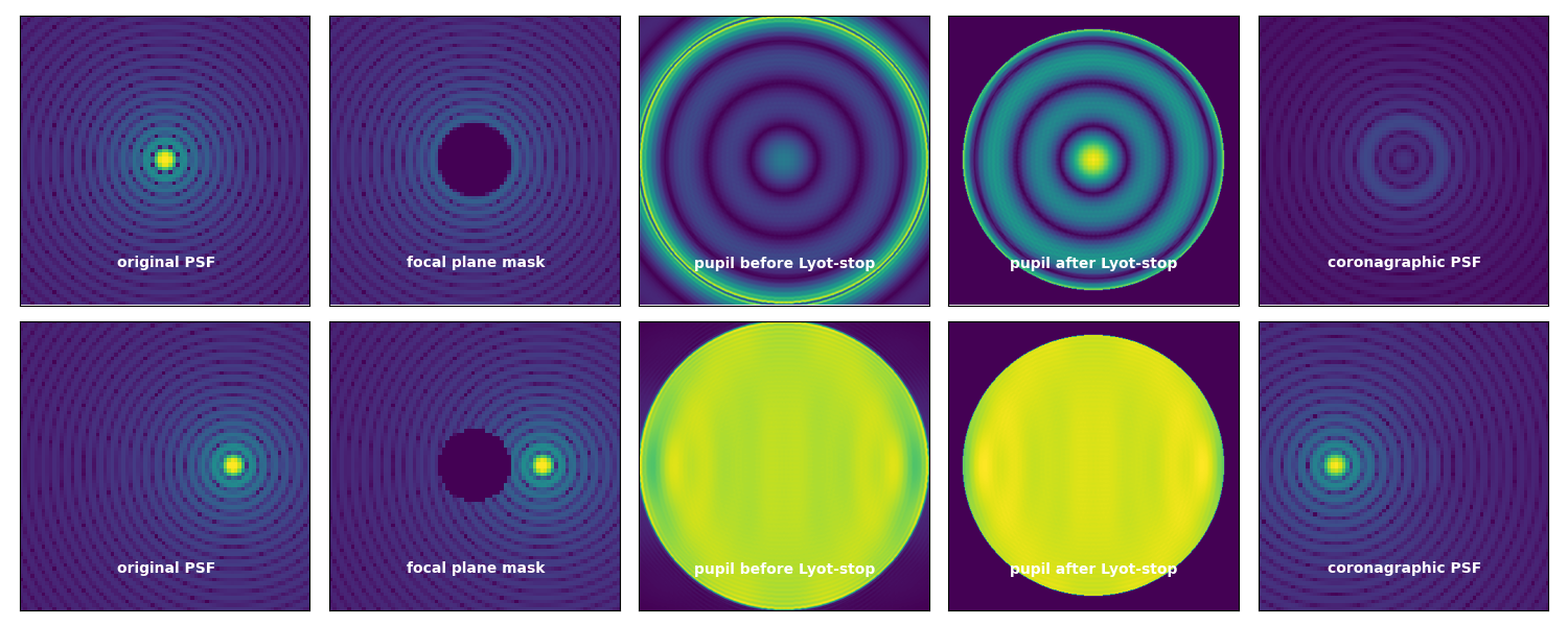
Illustration of the electric field (its modulus) as it goes through the different planes of a coronagraph. The top row shows what happens to an on-axis source, intercepted by the focal plane mask (second column of panels). The rest of the light is mostly diffracted (in the re-imaged pupil plane) near the edges of the aperture (third column of panels) and can be suppressed by an undersized Lot-stop (fourth row of panels). In the final focal plane (fifth column), the light of this on-axis source is considerably attenuated. The second row shows what happens to a source whose primary diffraction lobe misses the focal plane mask entirely.
5 Shack-Hartman camera
TBD!