How to account for field rotation
Table of Contents
1 Introduction
Unlike the venerable Palomar Hale Telescope that stands out as one of the last great telescopes to feature an equatorial mount, large telescopes use a more compact alt-azimuthal mount which means that as the telescope tracks a given target, if one were to lie down on the primary mirror, one would see the sky rotate. At the focus of an instrument that is at a fixed orientation relative to the pupil, the sky also rotates. Thus when tracking a star with companions as they transit, the companions will rotate around the primary.
It is possible to compensate for this apparent motion of the target that prevents the use of very long integrations, with a field derotator, but from the point of view of the camera, it is now the pupil of the telescope that rotates, and this will result in spinning diffraction features.
For high-contrast imaging, field rotation turns out to be a useful feature that makes it possible to easily disentangle the static diffraction features from actual companions. Full-aperture kernel-phase and sparse aperture closure-phase operate in fixed pupil mode, which means that they have to compose with sky rotation.
This page introduces how to use the XARA pipeline to account for field rotation when interpreting kernel-phase.
2 Detector position angle
When experiencing field rotation, the only way to make sense of the data being acquired at any instant is to keep track of the orientation of the detector relative to the true north, with an angle refered to as the detector position angle. In the software, the variable keeping track of this angle is called DETPA.
Assuming that one has been processing an image datacube with the XARA pipeline using the default cube extraction method (cf. example script), a look at the kpo1.DETPA variable would reveal an array filled with zeros: by default, the pipeline simply assumes that the detector pixels are aligned with the on-sky reference axis, with the north (N) pointing up and east (E) to the left, as is actually the case for PHARO images.
The convention used in the software is illustrated in the following image. The detector position angle DETPA is labeled ω and the companion position angle measured relative to the north is labeled \(\theta\).
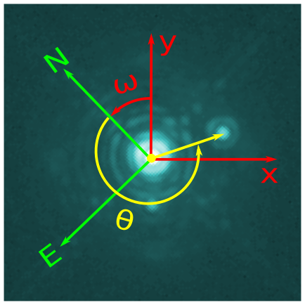
At the time of the extraction, the knowledge of the DETPA is not required: the only thing that matters is that you have a good, reliable discrete model that correctly accounts for all the features of the pupil. But when the time to interpret the data comes, such as when attempting to fit a binary kernel-phase model to the kernel-phase extracted from the datacube, then the proper DETPA info must be fed to the kpo data structure. Assuming the first data cube (index = 0) contains nim images, and that the known detector position angles are available in a distinct array called mydetpa, one can directly update the values using:
kpo1.DETPA[0] = mydetpa[:nim]
so that later, the call of kpo1.kpd_binary_model([sep, PA, con]) returns a list of arrays that matches the shape of the data acquired.
3 Simulating a dataset with field rotation
The following program uses the XAOSIM package to simulate a SPHERE SAM data-set in the K1 filter. XAOSIM features a preset for the AO system of GRAVITY that we can use here since SPHERE equips one of the VLT telescopes.
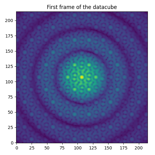
It saves a fits datacube of SAM interferograms recorded on a binary and (for the purpose of the demonstration) as the detector position angle varies continuously from 0 to 89 degrees… over 90 frames (1 additional degree of rotation per frame).
Note that no atmosphere or AO residuals are used here: the point of this tutorial is to see how field rotation affects the interpretation of kernel-phase.
Also note that we use XAOSIM but do not use its pseudo real-time features. In order to produce images, we need to do two things at each iteration:
make_image()updates the image on a shared memory data structureget_image()reads the data on the shared memory data structure and returns an array
import xaosim as xs
import numpy as np
from xaosim.pupil import SPHERE_IRDIS_SAM as sam
import astropy.io.fits as pf
import matplotlib.pyplot as plt

pscale = 12.255   # SPHERE IRDIS plate scale (mas/pixel)
cwavel = 2.11e-6  # K1 filter central wavelength (in meters)

try:
        _ = sphere.name
except NameError:
        sphere = xs.instrument("gravity", csz=480)
        sphere.cam2.update_cam(pscale=pscale, wl=cwavel)
        csz = sphere.csz
        ppscale = sphere.cam2.pdiam / csz  # pupil plate scale (meter/pixel)
        pupil0 = sphere.cam2.pupil.copy()  # the original pupil

sphere.cam2.update_cam(between_pixel=False)
sphere.cam2.pupil *= sam(csz)  # replacing the pupil by the SAM mask

# ----------------------------------------------------------------------
# prepare for later image crops: the cube built here is 215 x 215 pixels
# ----------------------------------------------------------------------

rsz = 215  # image size retained for cube
sphere.cam2.make_image()  # update simulation$
img0 = sphere.cam2.get_image()  # take an image
isz = img0.shape[0]  # image size

xy0 = (isz - rsz) // 2 + 1
xy1 = xy0 + rsz

imgc = img0[xy0:xy1, xy0:xy1]  # image cropped

# ----------------------------------------------------------------------
# properties of the simulated companion.
# ----------------------------------------------------------------------
sep = 115.  # separation (in mas)
PA = 257.0  # position angle (in degrees)
con = 0.1   # contrast (secondary/primary)

# ----------------------------------------------------------------------
# field rotation parameters: detector P.A. varies from 0 to 90 degrees
# ----------------------------------------------------------------------
nim = 90
detpas = np.arange(nim)
dcube = np.zeros((nim, rsz, rsz))

off_pointing = sphere.cam2.off_pointing  # short-hand!

# ----------------------------------------------------------------------
# simulating field rotation while observing the binary
# ----------------------------------------------------------------------
sep_pix = sep/pscale  # separation in # of pixels
for ii, detpa in enumerate(detpas):
        azim = (PA + detpa)*np.pi/180.0
        dx = -sep_pix * np.sin(azim)
        dy = sep_pix * np.cos(azim)
        sphere.cam2.make_image(phscreen=off_pointing(dx, dy))
                print("\r%04d: dra=%+6.2f, ddec=%+6.2f" % (ii, -dx, dy),
                  end="", flush=True)
        img1 = sphere.cam2.get_image()[xy0:xy1, xy0:xy1]
        dcube[ii] = imgc + con * img1

# save a datacube with a binary including rotation model
pf.writeto("sim_cube.fits", dcube, overwrite=True)

f1 = plt.figure(figsize=(5, 5))
ax1 = f1.add_subplot(111)
ax1.imshow(dcube[0]**0.2)
ax1.set_title("First frame of the saved datacube")
f1.set_tight_layout(True)
4 Kernel-phase interpretation of the dataset
To extract sensible kernel-phase out of the dataset that was just simulated, one first needs a model of the aperture. This is a sparse aperture masking dataset: there are more or less sophisticated ways of building models for one such dataset but we will stick to the simplest approach: our model will consist in only one sampling point per aperture.
4.1 Kernel-phase extraction
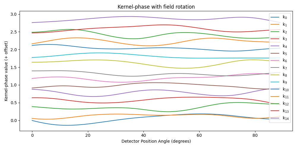
The coordinates of the seven holes of the SPHERE IRDIS SAM mask are used as input (coordinates taken from the source code of the pupil.SPHERE_IRDIS_SAM() function in the XAOSIM package source code) to build the model. These seven holes form 21 distinct baselines that can be assembled to form 15 kernel- or closure-phases.
With the detector plate scale and the wavelength of the filter in hand, the data cube can directly be processed and results in the compilation of 90 kernel-phase vector realisations, that all include the effect of a (thus far unaccounted for) varying detector position angle (DETPA).
import matplotlib.pyplot as plt
import numpy as np
import xara
import astropy.io.fits as pf
from xara.core import polar_coord_map as pcmap


# ==== KERNEL MODEL CREATION ====
mask_pos = 0.8 * np.array(
        [[+0.000, -3.9366],
         [-3.788, -1.7496],
         [+3.788, -1.7496],
         [-1.894, -0.6561],
         [-3.788,  0.4374],
         [-1.894,  3.7179],
         [+1.894,  3.7179]])

kpo1 = xara.KPO(array=mask_pos)

#  ==== KERNEL-PHASE EXTRACTION ====
tgt = pf.getdata("sim_cube.fits")
nim = tgt.shape[0]  # number of images
pscale = 12.255     # mas/pixel
cwavel = 2.11e-6    # central wavelength in meters

kpo1.extract_KPD_single_cube(tgt, pscale, cwavel)
data1 = np.array(kpo1.KPDT[0])
Because of the field rotation, we expect to see our 15 kernel-phases evolve over time, which is what the following snippet attempts to illustrate:
dmax = np.abs(data1).max()
nd = int(-np.round(np.log10(dmax)))
offset = np.round(dmax, nd)

f1 = plt.figure(figsize=(10, 5))
ax1 = f1.add_subplot(111)
for ii in range(kpo1.kpi.nbkp):
  ax1.plot(data1[:, ii] + offset * ii, label=r"k$_{%d}$" % (ii,))
ax1.legend()
ax1.set_xlabel("Detector Position Angle (degrees)")
ax1.set_ylabel("Kernel-phase value (+ offset)")
ax1.set_title("Kernel-phase with field rotation")
f1.set_tight_layout(True)
f1.savefig("kp_with_field_rotation.png")
4.2 Kernel-phase interpretation
In order to make sense of the data in the presence of field rotation, the KPO needs to know what is the value of the detector position angle (DETPA) for each frame. In practice, the DETPA would have to be extracted from the FITS header information that accompanies images produced by an instrument… or by additional byproducts of the early data massing software that a program usually relies on. Here, we know that the DETPA goes from 0 to 89 degrees in 1 degree increment and we can directly feed that to the KPO data structure.
4.2.1 1st guess: colinearity map
It is now possible to take advantage of a convenient kernel-phase investigation tool called the colinearity map. The following code snippet features one such use case: it computes a colinearity map over a 40 x 40 grid with a 10 mas step size. Wherever the signal recorded in the KPO data structure (present at index=0) matches the signal of a binary, the map peaks and a first estimate for the separation, position angle and contrast can be extracted from this first pass colinearity map. How close the result of this first estimate is from the expected value depends on the granularity of the map (here 10 mas).
kpo1.DETPA[0] = np.arange(nim)  # feed the DETPA!

gsize = 40  # grid size (gsize x gsize)
gstep = 10  # grid step in mas

mycomap = kpo1.kpd_colinearity_map(gsize, gstep, index=0)
f1 = xara.field_map_cbar(mycomap, gstep, vlabel="colinearity")
f1.suptitle("Signal colinearity map")

dist, azim = pcmap(gsize, gsize, scale=gstep)

x0, y0 = np.argmax(mycomap) % gsize, np.argmax(mycomap) // gsize
print("max colinearity found for sep = %.2f mas and ang = %.2f deg" % (
                dist[y0, x0], azim[y0, x0]))
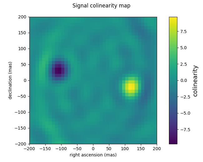
For this example, the thus far best solution is reasonably close to the values that were effectively simulated in the first place:
| Sep (mas) | PA (deg) | con | |
|---|---|---|---|
| Simulation input | 115 | 257 | 10 |
| Analysis output | 114.02 | 254.75 | 9.75 |
4.2.2 Correlation plot
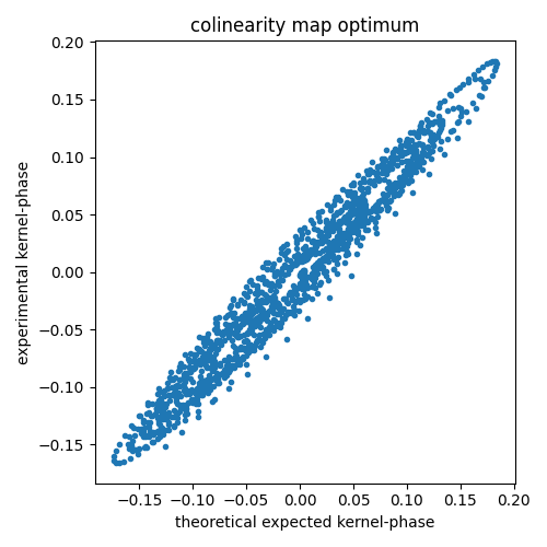
One other usual way of representing how this solution matches the actual dataset is to represent both in a correlation diagram. Building up from the above code, this how one could go about displaying this:
p0 = [dist[y0, x0], azim[y0, x0], mycomap.max()]
kmodel = kpo1.kpd_binary_model(p0)

f1 = plt.figure(figsize=(5, 5))
ax1 = f1.add_subplot(111)
ax1.plot(kmodel.flatten(), data1.flatten(), '.')
ax1.set_xlabel("theoretical expected kernel-phase")
ax1.set_ylabel("experimental kernel-phase")
ax1.set_title("colinearity map optimum")
f1.set_tight_layout(True)
f1.savefig("kp_field_rot_correlation_plot.png")
4.2.3 Further optimisation
The first estimate offered by the analysis of the colinearity map can serve as a first guess for an optimization procedure:
optim = kpo1.binary_model_fit(p0)
p1 = optim[0]  # best fit parameters
kmodel = kpo1.kpd_binary_model(p1)

f1 = plt.figure(figsize=(5, 5))
ax1 = f1.add_subplot(111)
ax1.plot(kmodel.flatten(), data1.flatten(), '.')
ax1.set_xlabel("theoretical expected kernel-phase")
ax1.set_ylabel("experimental kernel-phase")
ax1.set_title("colinearity map optimum")
f1.set_tight_layout(True)
f1.savefig("kp_field_rot_correlation_plot_2.png")
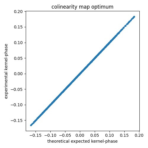
In this noise free case, the match between the solution and the data is of course perfect. Real world applications will of course not look as good as this ideal scenario! But at least, you should now feel able to tackle the kernel-phase analysis of data featuring field rotation!