PHARO data kernel-phase analysis example
Table of Contents
1 Introduction
This page features all of the code that was used for the analysis of the the P3K/PHARO dataset featured in the Martinache et al (2020) paper. This page should therefore be a good introduction into how to process your own datasets using XARA and the KERNEL project software tools in general.
2 PHARO medium-cross pupil mask model
Kernel-phase data analysis requires a decent model of the aperture. This dataset was acquired using a pupil mask called the medium-cross Lyot-stop so as to limit some of the flux for this fairly bright star α-Ophiucus. Pupil specifications for this mask are outlined in the Hayward et al (2001) paper describing the PHARO camera.
The script uses XAOSIM (another software product of the KERNEL project) to produce an image of the pupil of PHARO. To avoid rounding errors as much as possible in the creation of this pupil image that should be rotated 2 degrees to actually match the instrument pupil, the discrete representation of the aperture was computed with the spider veins aligned with the aligned with the main image axes.
After all (x,y) coordinates are computed, it is easy to get the right model by multiplying them by a rotation matrix. These coordinates, along with the unchanged pupil transmission model are what will serve as the basis to produce the kernel-phase model.
import numpy as np
import matplotlib.pyplot as plt
import matplotlib.cm as cm
import astropy.io.fits as pf
import xaosim as xs
from xaosim.pupil import PHARO
from scipy.ndimage import rotate
import xara

binary_model = False # use a finer transmission model for the aperture
PSZ     = 4978*2   # size of the array for the model
pdiam   = 4.978    # telescope diameter in meters
mstep   = 0.160    # step size in meters

pmask   = PHARO(PSZ, PSZ/2, mask="med")
pmask2  = PHARO(PSZ, PSZ/2, mask="med", ang=-2) # rotated!
ppscale = pdiam / PSZ

if binary_model:
        mtype="bina"
        p3k_model = xara.core.create_discrete_model(
                pmask, ppscale, mstep, binary=True, tmin=0.4)
else:
        mtype="grey"
        p3k_model = xara.core.create_discrete_model(
                pmask, ppscale, mstep, binary=False, tmin=0.05)
        p3k_model[:,2] = np.round(p3k_model[:,2],2)

# rotate the model by two degrees
# --------------------------------

th0 = -2.0 * np.pi / 180.0 # rotation angle
rmat = np.array([[np.cos(th0), -np.sin(th0)],
                                 [np.sin(th0), np.cos(th0)]])

p3k_model[:,:2] = p3k_model[:,:2].dot(rmat)

# -------------------------
#      simple plot
# -------------------------
f0 = plt.figure(0)
f0.clf()
ax = f0.add_subplot(111)
ax.imshow(pmask2)
ax.plot(PSZ/2+p3k_model[:,0]/ppscale,
                 PSZ/2+p3k_model[:,1]/ppscale, 'b.')
f0.set_size_inches(5,5, forward=True)

#f0.savefig("./imgs/PHARO/rotated_pupil.png")
# -------------------------
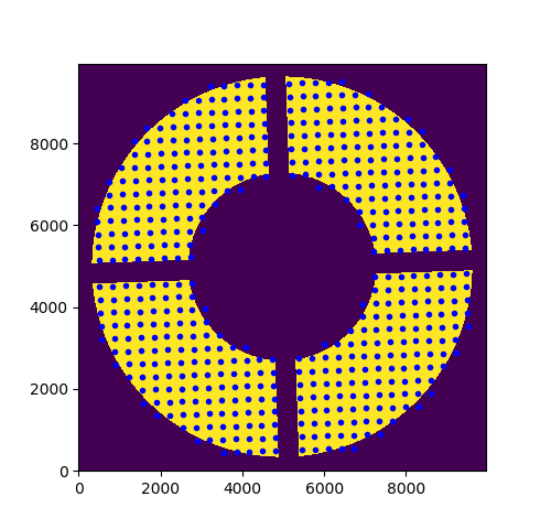
This image shows a high-fidelity (10,000 x 10,000 pixels!) image of the pupil rotated and the points overlaid show the location of the center of the virtual sub-apertures that will be used to produce the kernel-phase model of the PHARO data.
These (x,y) coordinates and the transmission function that is associated to each location are then used as input to compute the intial structure that will be used to do the kernel-phase analysis. The result is then saved as a multi-extension fits file such as described in the dedicated documentation page.
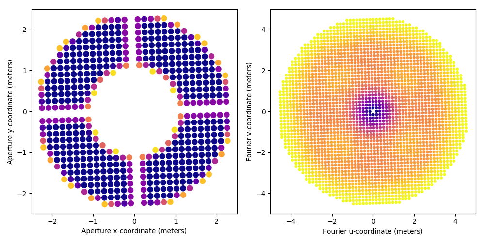
# compute the kernel-phase data structure
kpo_0 = xara.KPO(array=p3k_model, bmax=4.646)

# show side by side, the pupil model and its associated uv-coverage
kpo_0.kpi.plot_pupil_and_uv(xymax=2.5, cmap=cm.plasma_r, ssize=9, figsize=(10,5), marker='o')

# and save to a multi-extension kernel-phase fits file for later use
fname = "p3k_med_%s_model.fits" % (mtype,)
print("saving %s" % (fname,))
#kpo_0.save_as_fits(fname)
Traceback (most recent call last):
  File "<stdin>", line 1, in <module>
  File "/tmp/babel-2JWir0/python-dDdMfZ", line 2, in <module>
    kpo_0 = xara.KPO(array=p3k_model, bmax=4.646)
NameError: name 'p3k_model' is not defined
3 PHARO data-set kernel-phase analysis
3.1 Kernel-phase extraction
In order to be able to do the extraction of the Fourier-phase information, the software needs two additional pieces of information: what is the central wavelength of the filter used and what is the plate-scale of the camera. These two pieces of information make it possible to translate the model baselines, thus far computed in meters into radians, and to determine the parameters of the Fourier transform that is required to read the phase in the right place!
The script pre-loads two data-cubes containing 100 images of α-Oph and ε-Her (follow the links to download the data). As explained in the paper, these images were trimmed to 64x64 pixels.
import numpy as np
import matplotlib.pyplot as plt
import astropy.io.fits as pf
import xara

tgt_cube = pf.getdata('tgt_cube.fits') # alpha Ophiuchi
ca2_cube = pf.getdata('ca2_cube.fits') # epsilon Herculis

pscale = 25.0              # plate scale of the image in mas/pixels
wl     = 2.145e-6          # central wavelength in meters (Hayward paper)
ISZ    = tgt_cube.shape[1] # image size
kpo1   = xara.KPO(fname="p3k_med_grey_model.fits")
kpo2   = kpo1.copy()

kpo1.extract_KPD_single_cube(
        tgt_cube, pscale, wl,target="alpha Ophiuchi", recenter=True)
kpo2.extract_KPD_single_cube(
        ca2_cube, pscale, wl, target="epsilon Herculis", recenter=True)
3.2 Calibration of the kernel-phase
At this point, we have two complete kpo data structures, containing multiple kernel-phase measurements for both sources. Here, we'll simply average these multiple realizations of the kernel-phase vector and store the standard deviation of these realizations. The calibrated kernel-phase vector is the subtraction of the median kernel-phase obtained on the target of interest and that obtained on the calibration star. Some amount of error is added in quadrature to the experimental standard deviation so as to lead to a reduced χ2 = 1 at the later stages of this analysis.
data1 = np.array(kpo1.KPDT)[0]
data2 = np.array(kpo2.KPDT)[0]

mydata = np.median(data1, axis=0) - np.median(data2, axis=0)
myerr  = np.sqrt(np.var(data1, axis=0) / (kpo1.KPDT[0].shape[0] - 1) + np.var(data2, axis=0) / (kpo2.KPDT[0].shape[0] - 1))
myerr = np.sqrt(myerr**2 + 1.2**2)
3.3 Colinearity maps
In the high-contrast approximation, the kernel-phase signature of a binary companion is directly proportional to the contrast (using the secondary/primary convention). It is then somewhat covenient to look in the right ascension - declination parameter space surrounding the central object where the calibrated kernel-phase signal best mimics the signature of a companion. This is what the computation of a colinearity map achieves: for a finite number of laid out on a regular grid, one computes the theoretical signal that a contrasted companion would have, and then look at the result of the dot product between this prediction and the experimental kernel-phase. If a companion is present, the colinearity map will feature a maximum.
Note that due to the properties of kernel-phase that is sensitive to the presence of asymmetric features, the kernel-phase colinearity maps are always anti-symmetric.
print("\ncomputing colinearity map...")
gsize = 100 # gsize x gsize grid
gstep = 10 # grid step in mas
xx, yy = np.meshgrid(
        np.arange(gsize) - gsize/2, np.arange(gsize) - gsize/2)
azim = -np.arctan2(xx, yy) * 180.0 / np.pi
dist = np.hypot(xx, yy) * gstep

#mmap = kpo1.kpd_binary_match_map(100, 10, mydata/myerr, norm=True)
mmap = kpo1.kpd_binary_match_map(100, 10, mydata, norm=True)
x0, y0 = np.argmax(mmap) % gsize, np.argmax(mmap) // gsize
print("max colinearity found for sep = %.2f mas and ang = %.2f deg" % (
        dist[y0, x0], azim[y0, x0]))

f1 = plt.figure(figsize=(5,5))
ax1 = f1.add_subplot(111)
ax1.imshow(mmap, extent=(
        gsize/2*gstep, -gsize/2*gstep, -gsize/2*gstep, gsize/2*gstep))
ax1.set_xlabel("right ascension (mas)")
ax1.set_ylabel("declination (mas)")
ax1.plot([0,0], [0,0], "w*", ms=16)
ax1.set_title("Calibrated signal colinearity map")
ax1.grid()
f1.set_tight_layout(True)
f1.canvas.draw()
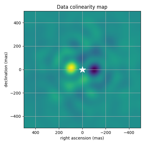
Colinearity map for the calibrated kernel-phase. A clear and unambiguous maximum is visible to the left of the primary, slightly less than 100 mas away from the center.
3.4 χ2 minimization
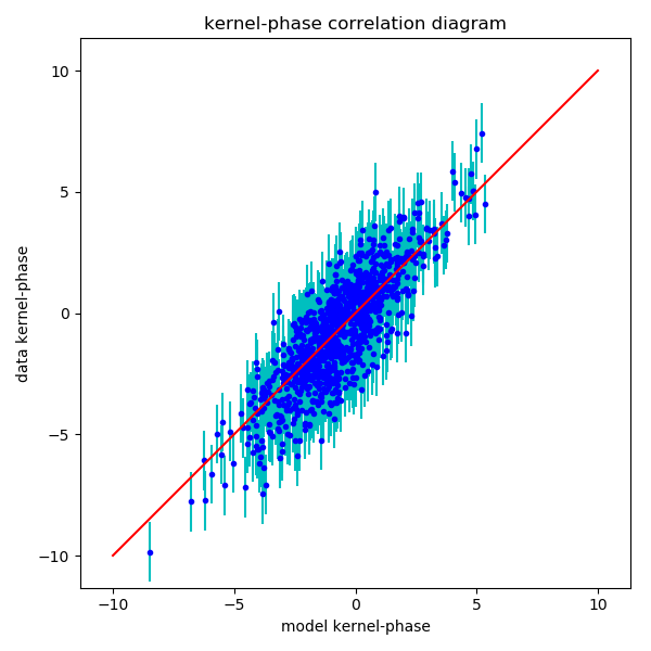
The solution identified at the previous stage makes for a very good first guess to be used by a traditional χ2 minimization procedure.
print("\nbinary model fitting...")
p0 = [dist[y0, x0], azim[y0, x0], mmap.max()] # good starting point

mfit = kpo1.binary_model_fit(p0, calib=kpo2)
p1 = mfit[0] # the best fit parameter vector (sep, P.A., contrast)

cvis_b = xara.core.cvis_binary(
        kpo1.kpi.UVC[:,0], kpo1.kpi.UVC[:,1], wl, p1) # binary
ker_theo = kpo1.kpi.KPM.dot(np.angle(cvis_b))

fig = plt.figure(figsize=(6,6))
ax = fig.add_subplot(111)

ax.errorbar(ker_theo, mydata, yerr=myerr, fmt="none", ecolor='c')
ax.plot(ker_theo, mydata, 'b.')
mmax = np.round(np.abs(mydata).max())
ax.plot([-mmax,mmax],[-mmax,mmax], 'r')
ax.set_ylabel("data kernel-phase")
ax.set_xlabel("model kernel-phase")
ax.set_title('kernel-phase correlation diagram')
ax.axis("equal")
ax.axis([-11, 11, -11, 11])
fig.set_tight_layout(True)

if myerr is not None:
        chi2 = np.sum(((mydata - ker_theo)/myerr)**2) / kpo1.kpi.nbkp
else:
        chi2 = np.sum(((mydata - ker_theo))**2) / kpo1.kpi.nbkp

print("sep = %3f, ang=%3f, con=%3f => chi2 = %.3f" % (p1[0], p1[1], p1[2], chi2))
print("correlation matrix of parameters")
print(np.round(mfit[1], 2))
4 Conclusion
This concludes the basic kernel-phase data analysis tutorial. Further analysis such as the determination of contrast detection limits would require the computation of covariance matrices. Refer to the dedicated page for more information on this topic.