Covariance & contrast detection limits
Table of Contents
1 Introduction
In the high-contrast regime, the kernel-phase signal of a binary companion is directly proportional to the secondary/primary luminosity ratio (contrast). The simple test that one can use in a given context to assess the detectability of a source of contrast \(c\) is the so-called "energy detector" that compares the energy (ie the square norm) of the kernel-phase binary signal to that of the uncertainty. How many times the energy of the signal is greater than the energy of the noise is going to quantify the strength of the detection (the number of σ). This page shows how to use a few of the XARA tools to compute 1-σ contrast detection limits based on this idea.
The first step to being able to determine these contrast detection limits is to compute the kernel-phase covariance matrix.
2 Covariance matrix
While kernel-phase have been designed to produce signals that are orthogonal to one another (a side product of the SVD), the noises affecting the initially independant pixels in the image result in covariated noises on the Fourier phase first, and then its projections onto the closure- and kernel-phase subspaces. To fully take this into account, one needs to keep track of the covariances in the system.
Noises (photon, readout, …) affect pixel measurements in the image. Let us assume that the noises affecting the different pixels are not covariated. This is valid for the photon noise (that follows Poisson statistics) and can be valid for the readout noise… depending on how the detector is actually read out.
2.1 Experimental covariance matrix
The most reliable way to compute the Fourier- and kernel-phase covariance matrix is of course to use a large dataset featuring enough statistical realisations of the noise to compute an experimental covariance matrix.
Assuming that you've processsed a datacube featuring enough images to enable the computation of a good covariance matrix, the following command:
kpo1.update_cov_matrix()
computes the experimental covariance for the Fourier-phase and the kernel-phase from the already processed data, and appends these two matrices to the kpo1 data structure:
kpo1.phi_covis the Fourier-phase covariance matrixkpo1.kp_covis the kernel-phase covariance matrix
If enough data is available, this is of course the ideal way to go.
2.2 Analytical covariance matrix
A first estimate of the photon-noise induced covariance can be computed using the pipeline. An instance of KPO gives access to a method called create_UVP_cov_matrix(var_img) that computes the covariance matrix using an analytical model that gives results that are a very good match to the experimental covariance when the level of noise is not too high.
The argument that must be passed to that function is a 2D representation of the variance of the noise affecting the image. In the photon-noise case following Poisson statistics for which the variance is equal to the mean, one simply feeds it an image, with the intensity adapted to match the total expected number of photons in the frame:
phi_cov = kpo1.create_UVP_cov_matrix(img0)
This function returns the Fourier-phase covariance matrix but also updates the two covariance matrices attached to the kpo1 data structure as described above. We will see this in action, using a simulated dataset that you might want to experiment with and adapt to the specifics of your scenario (telescope, camera, sparse aperture mask or not, …).
2.3 Simulated example
The following example uses the XAOSIM package to simulate a minimal dataset consisting of:
- a 2D representation of the pupil of the instrument
- an image by the Subaru/SCExAO instrument.
The pupil of the instrument is used to build a discrete model of the pupil, required for the kernel-phase analysis of the image. The image is used to compute analytical covariances for the Fourier and kernel-phase which are displayed afterwards.
import xara
import xaosim as xs
import numpy as np
import matplotlib.pyplot as plt

# create discrete model for SCExAO
# --------------------------------
PSZ = 792
pup = xs.pupil.subaru(PSZ, PSZ, PSZ/2, True, True)
pscale = 7.92 / PSZ
model = xara.core.create_discrete_model(
        pup, pscale, 0.3, binary=False, tmin=0.1)

kpo1 = xara.KPO(array=model, bmax=7.92)
kpo1.kpi.filter_baselines(kpo1.kpi.RED > 1)

# simulate an image by SCExAO
# ---------------------------
scexao = xs.instrument("scexao", csz=480)
img = scexao.snap()

# crop the image
# --------------
ysz, xsz = img.shape
rsz = 128
y0 = (ysz - rsz) // 2
x0 = (xsz - rsz) // 2

img0 = img[y0:y0+rsz, x0:x0+rsz]

# simulate photon noise
# ---------------------
img0 *= 1e7 / img0.sum()  # flux normalized to 1e7 photons
img0 = np.random.poisson(lam=img0)

# extract kernel-phase
# --------------------
pscale = scexao.cam.pscale  # plate scale in mas/pixel
cwavel = scexao.cam.wl      # central wavelength in meters
kpo1.extract_KPD_single_frame(img0, pscale, cwavel, target="SCExAO SIM")

# compute analytical covariances
# ------------------------------
_ = kpo1.create_UVP_cov_matrix(img0)

# display covariance matrices (non-linear display)
# ------------------------------------------------
f1 = plt.figure(figsize=(10, 5))
ax1 = f1.add_subplot(121)
ax1.imshow(np.arctan(kpo1.phi_cov*1e5))
ax1.set_title("Fourier-phase covariance")
ax1.set_xlabel("Baseline index")
ax1.set_ylabel("Baseline index")

ax2 = f1.add_subplot(122)
ax2.imshow(np.arctan(kpo1.kp_cov*1e2))
ax2.set_title("Kernel-phase covariance")
ax2.set_xlabel("Kernel index")
ax2.set_ylabel("Kernel index")

f1.set_tight_layout(True)
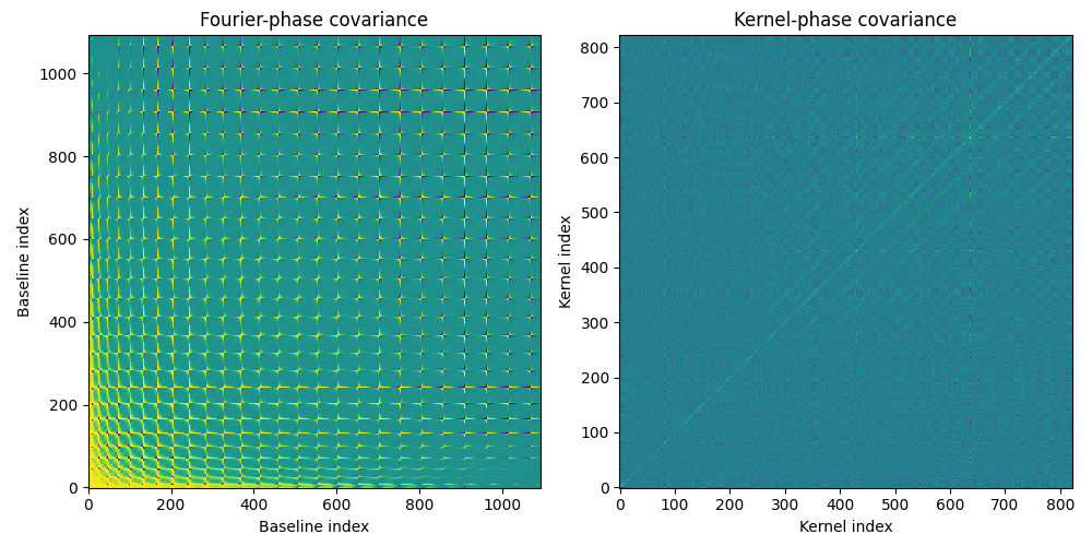
Without the non-linear arctan() scaling, the display of the Fourier-phase covariance reveals very little of its inner structure. The display uses a artcan because so as to avoid having to take the absolute value of the covariance. The checkered structure we see in the Fourier-phase covariance matrix is only due to the order in which baselines are accounted for in the discrete model. To get a feel for what the structure we see here actually means, we can attempt to reorder the baselines according to their length, which is what the following script achieves.
order = np.argsort(kpo1.kpi.BLEN)  # get the baselines length from the model
tmp = kpo1.phi_cov.copy()          # don't mess up the original covariance
tmp = tmp[order, :]                # reorder the covariance along the two axis
tmp = tmp[:, order]

f1 = plt.figure(figsize=(5, 5))
ax1 = f1.add_subplot(111)
ax1.imshow(np.arctan(tmp*1e5))
ax1.set_title("Fourier-phase covariance")
ax1.set_xlabel("Reordered baseline index")
ax1.set_ylabel("Reordered baseline index")
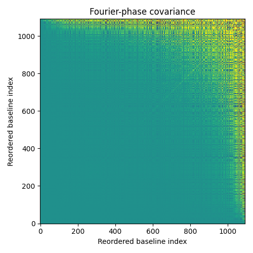
The reordering of the baselines according to their length does not absolutely guarantee continuity in the display but the overall trend of the magnitude of the covariance shows that it tends to increase with the baseline length. This effect is due not to the baseline length itself but more directly to the baseline redundancy: long baselines are less redundant and the Fourier phase of a low redundancy baseline is noisier than a highly redundant one (the central limit theorem is at work here).
While we can make somewhat insightful comments for the Fourier-phase, the kernel projection doesn't leave much chance to reveal anything interesting through the structure of the covariance.
3 Contrast detection limits
The kernel-phase covariance matrix can serve as the main input for an algorithm to compute contrast detection limits. The instance of KPO gives access to a method called kpd_binary_cdet_map that computes the contrast detection limits over a grid of positions specified by a grid size gsz and a grid step gstep specified in milliarcsecond.
3.1 Contrast detection limit map
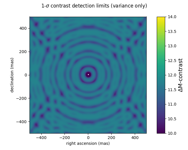
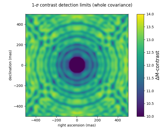
In the following example script, a 200x200 pixel grid contrast detection map with a 5 mas step (a total field of ± 500 mas) is computed using the analytical covariance matrix computed above, for 1e7 photons. The contrast detection maps are expressed in magnitude differences, at the 1-σ level. Pay attention to the difference between the two use cases: the first one uses only the diagonal of the covariance, and the second uses the whole covariance matrix. This reproduces the effect first described in Ireland (2013) when he suggests modifying kernel-phase to make them statistically independent.
gsz = 200
gstep = 5
cmag1 = kpo1.kpd_binary_cdet_map(gsz, gstep, np.diag(kpo1.kp_cov))
cmag2 = kpo1.kpd_binary_cdet_map(gsz, gstep, kpo1.kp_cov)

f1 = xara.field_map_cbar(cmag1, gstep, vmin=10, vmax=14,
                                                 vlabel="$\Delta$M-contrast")
f1.suptitle("1-$\sigma$ contrast detection limits (variance only)")

f2 = xara.field_map_cbar(cmag2, gstep, vmin=10, vmax=14,
                                                 vlabel="$\Delta$M-contrast")
f2.suptitle("1-$\sigma$ contrast detection limits (whole covariance)")
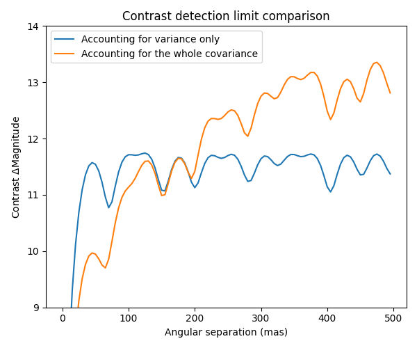
3.2 Contrast detection limit curve
A 1D cutout plot of these maps is also interesting to look at: it shows how using the variance only leads to uniform detection limits over the entire field of view. When taking the full covariance into account, the contrast detection limits increases with the angular separation.
f3 = plt.figure(figsize=(6,5))
ax3 = f3.add_subplot(111)
ax3.plot(np.arange(gsz//2)*gstep, cmag1[gsz//2, gsz//2:],
                 label="Accounting for variance only")
ax3.plot(np.arange(gsz//2)*gstep, cmag2[gsz//2, gsz//2:],
                 label="Accounting for the whole covariance")
ax3.set_xlabel("Angular separation (mas)")
ax3.set_ylabel("Contrast $\Delta$Magnitude")
ax3.legend()
ax3.set_title("Contrast detection limit comparison")
ax3.set_ylim([9, 14])
f3.set_tight_layout(True)