XARA data structures description
Table of Contents
1 Introduction
XARA manipulates two distinct data structures:
KPIstands for kernel-phase information. It contains the information that makes it possible to make sense of abstract data-sets such as kernel- and closure-phase. The same information also makes it possible to solve for the wavefront sensing problem when the virtual aperture (and its model) feature the appropriate properties. In the old NRM data reduction pipeline parlance, this is equivalent to a template.KPOstands for kernel-phase observation. It is most likely the only data structure that the end user directly manipulates and interacts with. It contains aKPIdata structure and the data that was extracted from images according to the information provided in theKPI.
2 KPI
A KPI data structure is effectively what is being computed when a Fourier-phase model is built from a discrete representation of the effective aperture of an imaging instrument. Assuming that one such discrete model is already available as an array (refer to the kernel model description page to see how to do just that), the KPI data structure is simply created calling:
import xara
my_kpi = xara.KPI(array=model, bmax=7.92)
The object contains several variables and numpy arrays that describe the virtual interferometric array.
2.1 KPI dimensions
Variables are introduced first since they are then use to describe the dimensions of the different numpy arrays:
| Variable | Mnemonic | Description |
|---|---|---|
my_kpi.nbap |
# of apertures | integer number of apertures in the virtual pupil array |
my_kpi.nbuv |
# of uv coordinates | integer number of virtual baselines |
my_kpi.nbkp |
# of kernel-phases | integer number of kernel-phases |
The number of kernels nbkp (\(n_K\)) depends on the rank of the baseline mapping matrix described below. The values these variable take do reflect the properties of the geometry of the virtual array. If the aperture is 180-degree rotational symmetric, the number of kernels nbkp = nbuv - nbap/2 (\(n_K = n_B - n_A / 2\)). If not, the number of kernel decreases nbkp = nbuv - nbap (\(n_K = n_B - n_A\)) to the benefit of the number of eigen-phases. The decrease in the number of kernels means that baseline-mapping and phase-transfer matrices (described below) become fully invertible and can be used for wavefront retrieval.
2.2 KPI arrays
| Array | Mnemonic | Dimension | Description |
|---|---|---|---|
my_kpi.VAC |
Virtual Array Coordinates | nbap x 3 | 3 column description (coordinates in meters + transmission) of the virtual array fed to the constructor |
my_kpi.TRM |
TRansmission Model | nbap x 1 | contains the transmission of the virtual array (identical to my_kpi.VAC[:,2] |
my_kpi.UVC |
UV Coordinates | nbuv x 2 | coordinates of the baselines (in meters) of the model |
my_kpi.RED |
REDundancy | nbuv x 1 | redundancy associated to the baselines |
my_kpi.BLM |
BaseLine mapping Matrix | nbuv x nbap | matrix describing how virtual sub-apertures contribute to the different baselines |
my_kpi.TFM |
TransFer phase Matrix | nbuv x nbap | matrix describing the way the pupil phase relates to the uv-phase |
my_kpi.KPM |
Kernel-Phase Matrix | nbkp x nbuv | Kernel of the Transfer phase matrix |
The BLM and the TFM are related as follows:
TFM = np.diag(1./RED).dot(BLM)
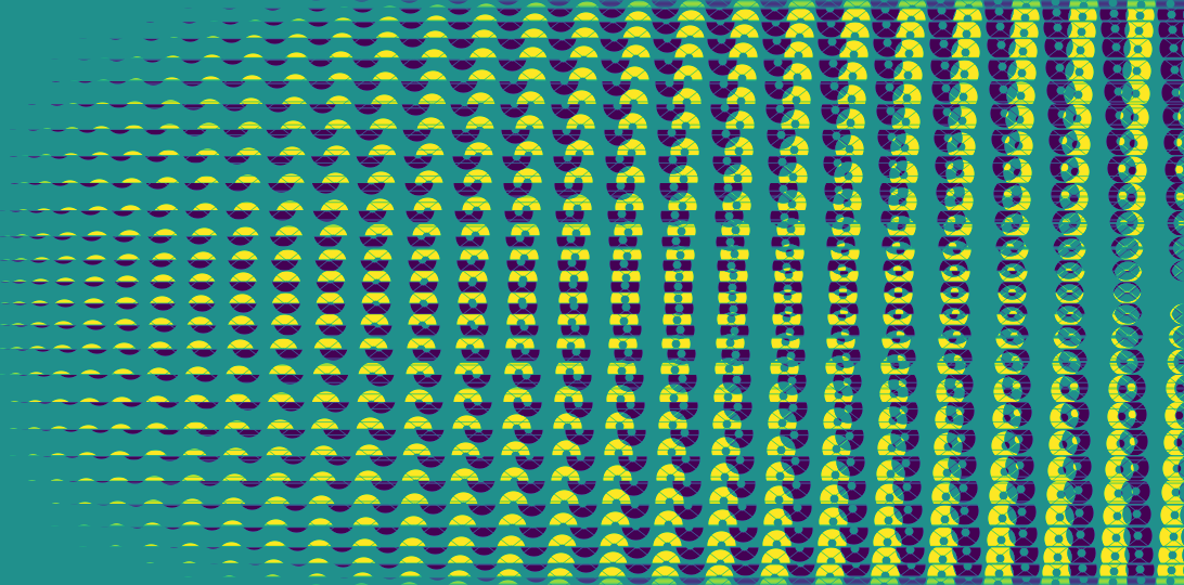
BLM is an unweighted representation of the contribution of the virtual sub-apertures to the different baselines. Unlike the TFM, it can be visualized and here is what the BLM of the grey example featured in the model creation part of the documentation looks like (transposed for a "landscape" feel):
plt.imsave("BLM_Subaru_grey_30cm.png", my_kpi.BLM.T) # transposed
2.3 Saving the KPI data structure
The thus constructed KPI data-structure can be saved as a multi-extension fits file to be later recalled, for instance prior to extracting kernel-phases from an image into a KPO data-structure.
my_kpi.save_as_fits("my_kernel_model.fits.gz")
3 KPO
3.1 creation
A KPO data-structure is created from scratch almost exactly like a KPI, using the following constructor call:
import xara
my_kpo = xara.KPO(array=model, bmax=7.92)
which also computes a KPI data structures that is appended to my_kpo (actual instance is my_kpo.kpi). It can be reloaded from a previously saved data-structure:
import xara
my_kpo = xara.KPO(fname="my_kernel_model.fits.gz")
which produces the following output:
Attempting to load file my_kernel_model.fits.gz
KPI data successfully loaded
The file contains 0 data-sets
CWAVEL was not set
No covariance data available
informing the user that the KPI data-structure was well loaded, but that no data-set (kernel-phase) was found.
Attributes and methods of the KPI can be directly accessed as shown in the following examples:
# plots the properties of the discrete model
my_kpo.kpi.plot_pupil_and_uv(xymax=4.0, cmap=cm.plasma_r, ssize=9, figsize=(10,5), marker='o')

# outputs the number of kernels one is to expect from this model
print("# of kernels = %d" % (my_kpo.kpi.nbkp,))
3.2 appending data
The purpose of the KPO data structure is of course to include actual data extracted from images. The information contained in the KPI data-structure alone is not sufficient to extract meaningful Fourier information from an image: one must additionally provide at least the plate-scale pscale of the detector and the central wavelength CWAVEL of the filter used. This information, along with the orientation of the detector relative to the sky (DETPA) and the time the data was acquired (MJDATE) that will be used to later interpret the astrophysical meaning of the kernel-phase data can often be found in the FITS files headers containing the data.
Initially, XARA attempted to implement a certain number of pre-sets for different instruments. Although arguably convenient, the code of these presets is not very interesting to write and read so instead, the recommendation is to leave some of the house-keeping to the user. Two generic functions:
extract_KPD_single_frameextract_KPD_single_cube
are now the prefered way of extracting the data: the plate-scale and the wavelength must be provided explicitly. The following replicates some of the information already available in the kernel data-analysis overview page.
import xara
import astropy.io.fits as pf

# load the images
img = pf.get_data("my_image.fits")
cub = pf.get_data("my_cube.fits")

# creation of the KERNEL model from a text-file describing the virtual array
cal1 = xara.KPO(fname="my_discrete_model.txt")

# image kernel-extraction
pscale = 16.7   # plate scale of the image          (in mas/pixel)
wl     = 1.6e-6 # wavelength the image was acquired (in meters)

# extracting a single realisation into cal1
cal1.extract_KPD_single_frame(img, pscale, wl, target="The Banana Star", recenter=True)

# extracting multiple realisations into cal2
cal1.extract_KPD_single_cube(cub, pscale, wl, target="My UFO video", recenter=True)

# saving the result as a kernel FITS file
cal1.save_as_fits("my_kernel_data_set.fits")
The two data-sets have been appended to a single KPO structure. Each extraction call appends data (complex visibility CVIS and kernel-phase KPDT) to a list.
3.3 resulting data structures
| Data-structure | Mnemonic | Description |
|---|---|---|
cal1.FF |
Fourier | Complex DFT matrix |
cal1.CVIS |
Complex Visibility | list of complex visibilities |
cal1.KPDT |
Kernel-Phase DaTa | list of kernel-phase |
cal1.MJDATE |
Modified Julian DATE | list of dates matching individual frames |
cal1.DETPA |
Detector Position Angle | list of detector orientation matching frames |
3.4 Saving the KPO data structure
The resulting KPO data-structure can be saved as a multi-extension fits file to be shared with kernel-phase afficionados all around the world.
cal1.save_as_fits("my_kernel_data.fits.gz")
At the moment, only the kernel-phase (KPDT) information is actually written to file. The complex visibility (CVIS) is not currently preserved although this is likely to change if instruments featuring stable visibilities find a use for them.