Kernel-analysis model creation
Table of Contents
1 Discrete models
Kernel-phase analysis processes images as if they were the result of a virtual discrete grid of sub-aperture forming together an interferometer with a dense (but adjustable) aperture. This discrete representation of the continuous reality makes it possible to assemble observables that are naturally resilient to second order instrumental phase error in the pupil.
The end result is either a 2-column (x,y) or a 3-column (x,y,t) array of variables respectively representing the horizontal (x) and vertical (y) position of the virtual sub-aperture (both in meters) and an optional dimension-less transmission function t, associated to this virtual sub-aperture.
2 Creation of a discrete model using XARA
The XARA pipeline offers the means to create a discrete model reasonably simply, from a 2D description of the pupil of an instrument and a scaling parameter.
The following example uses another package also maintained in the context of the KERNEL project called XAOSIM, to generate the 2D array describing the aperture of a telescope (here the Subaru Telescope).
The important function call is xara.core.create_discrete_model(), the documentation of which the user is strongly encouraged to refer to. Up until the second part of 2019, discrete models used in practice were of a binary nature, i.e. each virtual sub-aperture of the model is either fully transmissive or discarded. Recently, XARA has introduced the possible use of a local transmission function to better reflect the fine structures of the pupil without having to resort to a super fine paving of the aperture.
2.1 Binary aperture model creation example
#!/usr/bin/env python
import xara
import xaosim as xs

PSZ = 792
pup = xs.pupil.subaru(PSZ, PSZ, PSZ/2, True, True)
pscale = 7.92 / PSZ
model = xara.core.create_discrete_model(pup, pscale, 0.3, binary=True, tmin=0.5)
The Subaru Telescope pupil is of diameter 7.92 meters. We use XAOSIM to create a 792x792 array, therefore describing the Subaru Telescope pupil with a 1 cm per pixel scale (the pscale parameter). We create the model with a grid step size of 0.3 meter (30 cm), and request a binary model, where each sub-aperture is either 100 % or 0 % transmissive. The cut-off value marking the difference between transmissive or not is set to tmin=0.5, which is where one seems to get the best results for a binary model.
The result is a 3-column array, here with 508 rows, as shown in the following printout:
array([[-0.6, -3.9,  1. ],
       [-0.3, -3.9,  1. ],
       [ 0. , -3.9,  1. ],
       ...,
       [ 0. ,  3.9,  1. ],
       [ 0.3,  3.9,  1. ],
       [ 0.6,  3.9,  1. ]])
2.2 Grey model creation example
This is now the recommended way of creating a discrete aperture model: for a given grid size, the overall fidelity of the Fourier-phase model is improved typically by one order of magnitude. The major difference with the earlier scenario is the use of the False option for the binary flag, and a more permissive transmission cut-off value. Your use case may require you to produce a finer pupil image (and an adjusted pscale value) as an input to the model creation function.
#!/usr/bin/env python
import xara
import xaosim as xs

PSZ = 792
pup = xs.pupil.subaru(PSZ, PSZ, PSZ/2, True, True)
pscale = 7.92 / PSZ
model = xara.core.create_discrete_model(pup, pscale, 0.3, binary=False, tmin=0.1)
3 Creation of a kernel model using XARA
Once this model created, it can either be saved as a text file, using for instance the following numpy function call (with enough significant digits):
import numpy as np
np.savetxt("my_discrete_model.txt", model, fmt="%+.6e %+.6e %.2f")
Before being used as argument when creating either a KPI (Kernel-phase information) or a KPO (Kernel-phase object), using either of these two approaches:
import xara

# if the model is already loaded
cal = xara.KPO(array=model, bmax=7.92)

# if the model needs to be reloaded from a previously saved fits file
cal = xara.KPO(fname="my_discrete_model.txt", bmax=7.92)
Depending on the complexity of the virtual discrete representation of the aperture, the actual computation of the model can take some time. A discrete representation with up to a 1000 virtual sub-apertures in the pupil will likely suffice most needs and should take less than a minute on a not particularly recent computer.
If you pay attention to the KPO object creation call, you will see that an optional bmax parameter was provided and requires some further explanations. At the earlier step of the creation of the discrete aperture model, especially when using a grey model, one cannot exclude the possibility that virtual baselines produced by one such model will end up being slightly larger than the true aperture diameter. The bmax option is a safeguard that tells the KPO data structure creation function to discard any resulting baseline that would be greater than the provided value (here set to 7.92 meters, ie. the original aperture diameter). In some very low SNR cases, it may be useful to discard baselines more agressively. Some of the higher spatial frequency information potentially available in the image will be lost but so will be the higher noise that comes with them.
3.1 Saving and visualizing the properties of a discrete Fourier phase model
Once computed, the data structure can be saved as a multi-extension fits file for faster recall. XARA offers a convenient model plot utility:
cal.kpi.plot_pupil_and_uv(xymax=4.0, cmap=cm.plasma_r, ssize=9, figsize=(10,5), marker='o')
that gives a pretty good idea of what the discrete representation of the aperture feels like (on the left) and what uv-coverage (on the right) this model theoretically gives access to. The result of the two computations are shown below, first for the binary model:
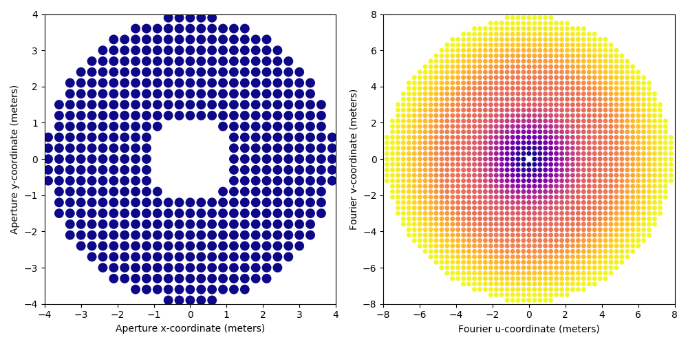
And then for the grey model:
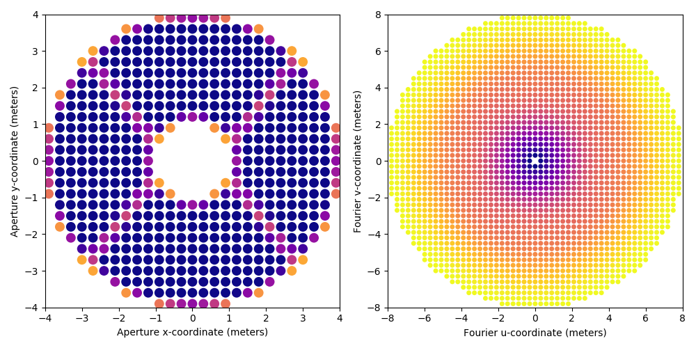
Note that although the two models use the same grid size and thefore result in matrices of comparable sizes, the grey model better reflects the finer structures of the aperture.
Refer to the documentation of plot_pupil_and_uv to taylor its output to your actual needs. It turns out to take a few steps to produce a png figure that looks all right without disturbing aliasing effects.