JWST Brown-Dwarf data analysis
Table of Contents
1 Context
1.1 Description of the data
Simulated NIRISS F480M images provided by Alex Greenbaum.
- Files in BRIGHT correspond to brighter sources like WISE 1405+5534 W2mag=14.097, simulated with 1.2e7 counts in ~40 min
- Files in FAINT correspond to sources like WISE 0359-5401 W2mag = 15.384, at 4e6 counts in ~40 min
- Files with tbinary in the name contain the companion signal. Files with cbinary are a "calibrator" source without the companion signal. You will see that there are 4 contrasts from 0.1 to 0.01 simulated at ~lam/D and ~lam/2D (one position angle).
- Files in the NOISELESS directory are generated just by convolving the PSF with the same sky scene and without adding noise. There is some noise in generating the PSF (OPD, jitter) but no detector/photon noise. There is also a single PSF included in this directory.
- At top level there is the NIRISS CLEARP mask from webbpsf "MASKCLEAR.fits.gz"
- images are 81x81 pixel.
1.2 General philosophy
- Kernel-phase is not a deconvolution technique, since deconvolution remains an ill-posed problem. Instead, we place ourselves in a restricted information space that is untouched by residual pupil-phase aberrations.
- One such sub-space exists in the phase part of the Fourier transform of images.
- to find this space, we pretend that the data was produced by a discrete aperture and we build a representation of the way the aperture phase noise propagates into spurious phase information in the Fourier plane
- this model is a linear operator that encodes our understanding of the aperture that diffracts, and includes the possible redundancy of the aperture
- build kernel-phases by looking at the properties of the linear operator
- For a given model, when looking at a binary object, the amplitude of the signal is proportional to the contrast of the companion.
- Kernel-phases however remain an abstract quantity. To understand what it means goes beyond even what students sometimes call the Fourier Vision superpower. Just use kernel-phase as input to some kind of model-fitting algorithm.
2 Discrete models
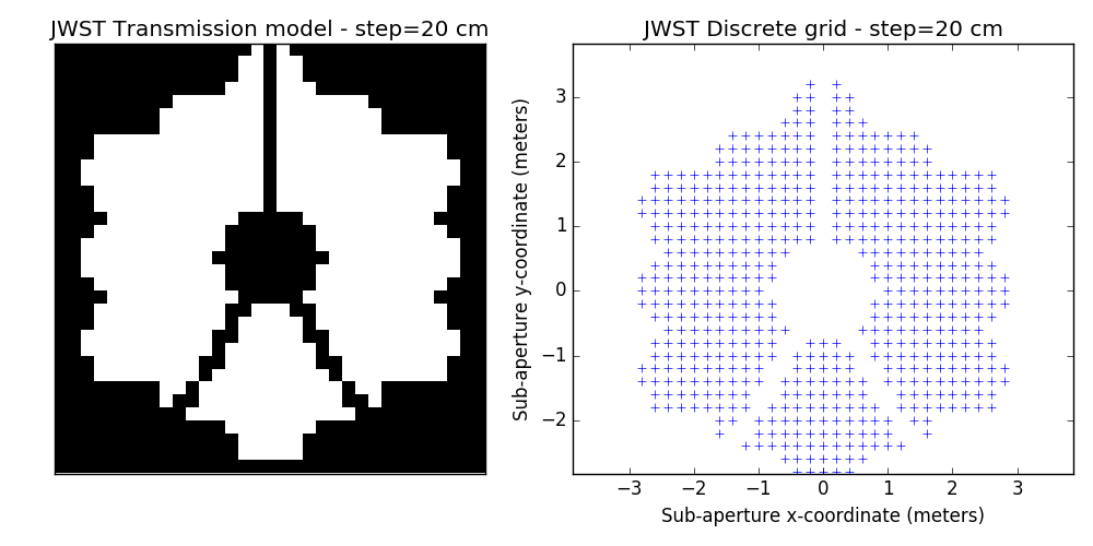
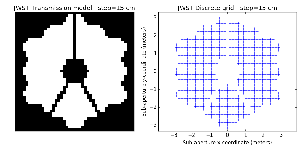
Discrete models are built from a regular square grid of points. Although the aperture of JWST is hexagonal, the analysis sticks to square grid, which in practice (after a fair bit of experimentation) is more computationally efficient and less prone to errors.
At the moment, the grid is binary: either the point is included or it is excluded from the model. There have been attempts with grey descriptions of the aperture. They don't seem to bring much to the table yet, but things may change in the future. The python program provided below for reference can generate both gray and binary models.
2.1 discrete model generation algorithm
#!/usr/bin/env python

import numpy as np
import matplotlib.pyplot as plt
import matplotlib.cm as cm
from astropy.io import fits

# ============================
#   script parameters
# ============================
step    = 0.15                             # grid step size in meters
thr     = 5e-1                             # selection threshold for mask
binary  = True                             # binary or grey mask
blim    = 0.9                              # threshold for binary mask

# ============================
#      begin script
# ============================
hdul    = fits.open('MASKCLEAR.fits.gz')
apert   = hdul['PRIMARY'].data
ppscale = hdul['PRIMARY'].header['REALSCAL'] # pupil pixel size in meters
PSZ     = apert.shape[0]                     # pupil image size


nbs     = int(PSZ / (step / ppscale))        # number of sample points across

if not (nbs % 2):
        nbs += 1 # ensure odd number of samples (align with center!)

# ============================
#   pad the pupil array
# ============================

PW      = int(step / ppscale) + 1            # padding width
padap   = np.zeros((PSZ+2*PW, PSZ+2*PW))     # padded array
padap[PW:PW+PSZ, PW:PW+PSZ] = apert
DSZ     = PSZ/2 + PW

# ============================
#  re-grid the pupil -> pmask
# ============================

pos = step * (np.arange(nbs) - nbs/2)
xgrid, ygrid = np.meshgrid(pos, pos)
pmask = np.zeros_like(xgrid)

xpos = (xgrid / ppscale + DSZ).astype(int)
ypos = (ygrid / ppscale + DSZ).astype(int)

for jj in range(nbs):
        for ii in range(nbs):
                x0 = int(xpos[jj,ii])-PW/2
                y0 = int(ypos[jj,ii])-PW/2
                pmask[jj,ii] = padap[y0:y0+PW, x0:x0+PW].mean()

# ==========================
#  build the discrete model
# ==========================

xx = [] # discrete-model x-coordinate
yy = [] # discrete-model y-coordinate
tt = [] # discrete-model local transmission


if binary is True:
        for jj in range(nbs):
                for ii in range(nbs):
                        if (pmask[jj,ii] > blim):
                                pmask[jj,ii] = 1.0
                                xx.append(xgrid[jj,ii])
                                yy.append(ygrid[jj,ii])
                                tt.append(1.0)
                        else:
                                pmask[jj,ii] = 0.0

else:
        for jj in range(nbs):
                for ii in range(nbs):
                        if (pmask[jj,ii] > thr):
                                xx.append(xgrid[jj,ii])
                                yy.append(ygrid[jj,ii])
                                tt.append(pmask[jj,ii])

xx = np.array(xx)
yy = np.array(yy)
tt = np.array(tt)

model = np.array([xx, yy, tt]).T
np.savetxt("jwst_model.txt", model, fmt="%+.6e %+.6e %.2f")

# =================================================
fx, (ax1, ax2) = plt.subplots(1,2)
fx.set_size_inches(10, 5, forward=True)
ax1.imshow(pmask, origin="lower", interpolation="nearest", cmap=cm.gray)
ax1.set_xticks([])
ax1.set_yticks([])
ax1.set_title('JWST Transmission model - step=%2d cm' % (step*100,))

ax2.plot(xx, yy, 'b+')
ax2.axis('equal')
ax2.set_title('JWST Discrete grid - step=%2d cm' % (step*100,))
ax2.set_xlabel("Sub-aperture x-coordinate (meters)")
ax2.set_ylabel("Sub-aperture y-coordinate (meters)")
fx.set_tight_layout(True)
# =================================================
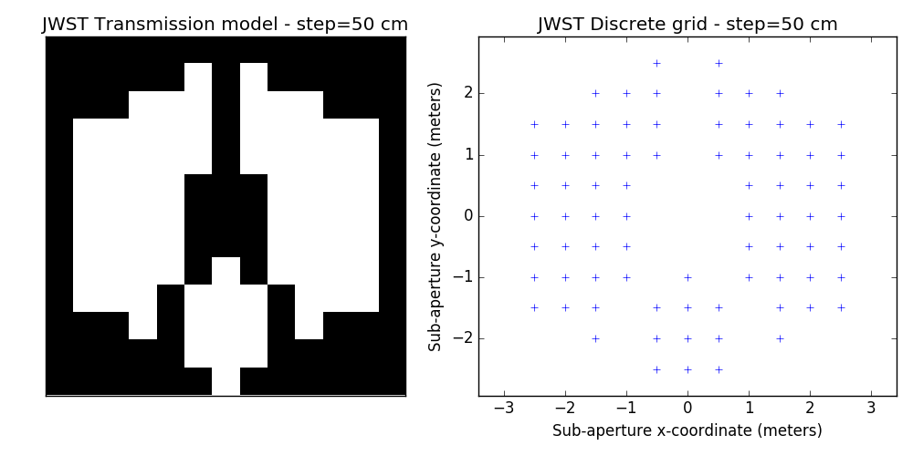
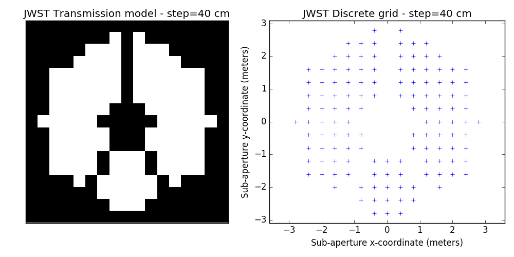
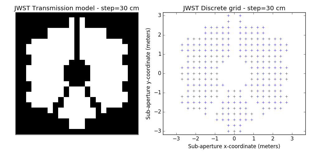
2.2 examples of discrete binary models
One tunable parameter is the grid size. A few examples are illustrated here and will be used in the analysis described further. The different values for the grid size parameter are: 50 cm, 40 cm, 30 cm, 20 cm and 15 cm. The finer the grid, the more visually satisfying the model becomes. This however comes at a cost: the linear model grows in complexity and the computation of the SVD used to determine kernel-phase relations for the model can become time-consuming.
3 Noise-free case
3.1 analysis script
#!/usr/bin/env python

import numpy as np
import matplotlib.pyplot as plt
import matplotlib.cm as cm
import xara

plt.ion()
plt.show()

sep = 147.0
pa = 45.0
con = 0.1

cal0  = xara.KPO(fname="jwst_model_0.15.txt")
calib = cal0.copy()
trgt1 = calib.copy()

suffix = "_CLEARP_F480M_opd_req_bb250K.fits"
calib.extract_KPD("./noiseless/F480M/PSF_det"+suffix,
                                 target="PSF")

trgt1.extract_KPD(
        "./noiseless/F480M/binary_s147.0_p45.0_cr0.1.fitsPSF_15ov"+suffix,
        target="binary")

kp_model  = calib.kpd_binary_model([sep, -pa, 1./con], index=0, obs="KERNEL")[0]
kp_signal = trgt1.KPDT[0][0] - calib.KPDT[0][0]

error = kp_signal - kp_model
print("error on c=0.1 model = %.2f mrad rms" % (error.std() * 1e3,))

print("----------------------------")
print("error = %.2f mrad"  % (error.std() * 1e3, ))
print("signl = %.2f mrad"  % (kp_signal.std() * 1e3, ))
print("calib = %.2f mrad"  % (calib.KPDT[0][0].std() * 1e3, ))
print("----------------------------")

# ===========================================================================
# ===========================================================================
fx, (ax1, ax2) = plt.subplots(1, 2, gridspec_kw = {'width_ratios':[1, 0.6]})
fx.set_size_inches(15,6, forward=True)

offset = np.round(2*kp_model.std())

ax1.plot(trgt1.KPDT[0][0]+offset, 'b', label="raw binary kernel")
ax1.plot(calib.KPDT[0][0]+offset, 'y', label='raw calibrator kernel')
ax1.plot(kp_signal-offset,        'r', label='calibrated kernel')
ax1.plot(kp_model-offset,         'g--', label='binary model kernel')
ax1.set_xlabel('Kernel-phase index', fontsize=11)
ax1.set_ylabel('Kernel-phase (radians)', fontsize=11)
ax1.set_xlim(0, calib.kpi.nbkp)
ax1.legend(fontsize=11)


ax2.plot(kp_model, kp_signal, 'b.')
ax2.set_ylabel('Calibrated Kernel-phase data (radians)', fontsize=11)
ax2.set_xlabel('Kernel-phase 10:1 model (radians)', fontsize=11)
ax2.grid()
fx.set_tight_layout(True)
3.2 plot of analysis result
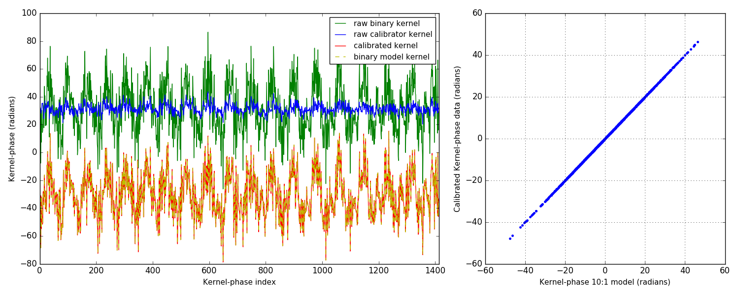
3.3 comment of the plot
From the plot on the right, you can tell that things are looking pretty good. Simulations are so much better than the real thing, isn't it? Couple of things to point out: I only show the easiest scenario: 10:1 companion at ∼ 1 λ/D. Other simulations in the noise-free case are all similar and the calibrated kernel-phase signal almost perfectly matches the expected signature from a model.
On the left, the different plots show something more: four curves are represented, with offsets applied so as to make them easier to read. The green curve is the raw kernel-phase signal recorded on the binary alone. The blue one is the raw kernel-phase signal recorded on the point source: this is the kernel-phase bias, which if everything was perfect should be zero. The simulated PSF is however not perfect, and notably includes the effect of jitter, which smears the PSF ever so slightly. Part of this also comes from the discretization error that also translates into a bias. Both effects result in kernels that do not go to zero when looking at a point source. This is why calibration is important.
For this 10:1 contrast companion, the amplitude of the signal is significantly larger than that of the bias, so it could be found even without calibrating, albeit biased and/or with larger uncertainties on the parameters of the fit. However since the amplitude of the binary signature is proportional to the contrast, it can become dominated by the kernel-phase bias.
The final two curves show the calibrated kernel-phase signal compared to the expected kernel-phase signature of a companion in the right place. The match is near perfect, as further shown by the correlation plot on the right.
4 Noisy data-sets
This analysis is a first-pass, destined to give us a starting point, which can and will be improved upon. Two refinements will play a part:
- improved discrete models. This is a bit prospective: we are looking into ways to better model fine details of the aperture: edges and spider vanes (what we call grey models). The results shown here are for the discrete model with the finest grid shown above (15cm)
- use of covariance matrices to decorrelate the effects of noise. This is a demonstrated way of improving contrast detection limits (see below). It has not been used for this first pass. Given that photon noise clearly dominates here (see contrast curves below), this procedure is expected to have a major impact on the final performance.
Two types of data-sets were provided: bright and faint. Companions were simulated for two angular separations (73.5 mas and 147.0 mas, which roughly correspond to λ/D and 0.5λ/D) and for contrasts ranging between 10:1 and 100:1.
Finally: it seems the errors, solely estimated from the kernel-phase scatter from frame to frame (15 per data-cube) are over-estimated (by a factor of 3?), as the observed reduced χ2 of all data fit is ∼ 0.1. We will see how this goes after implementing the noise decorrelation procedure.
4.1 analysis script
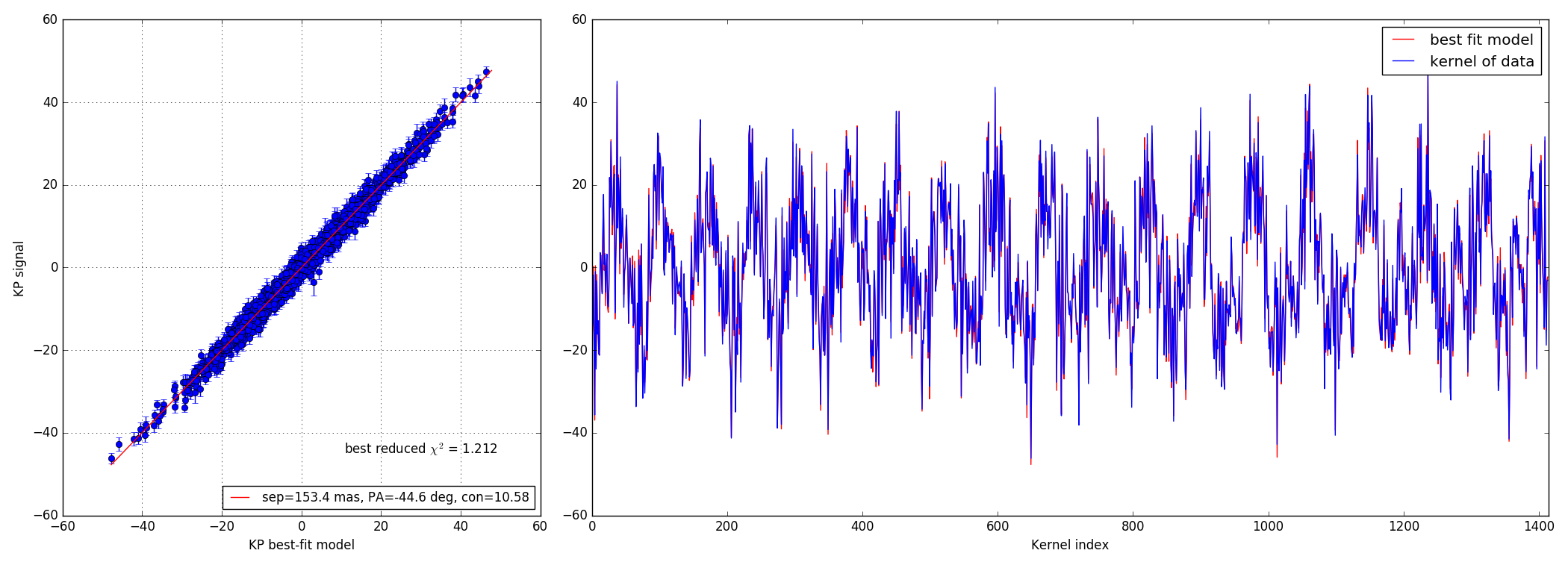
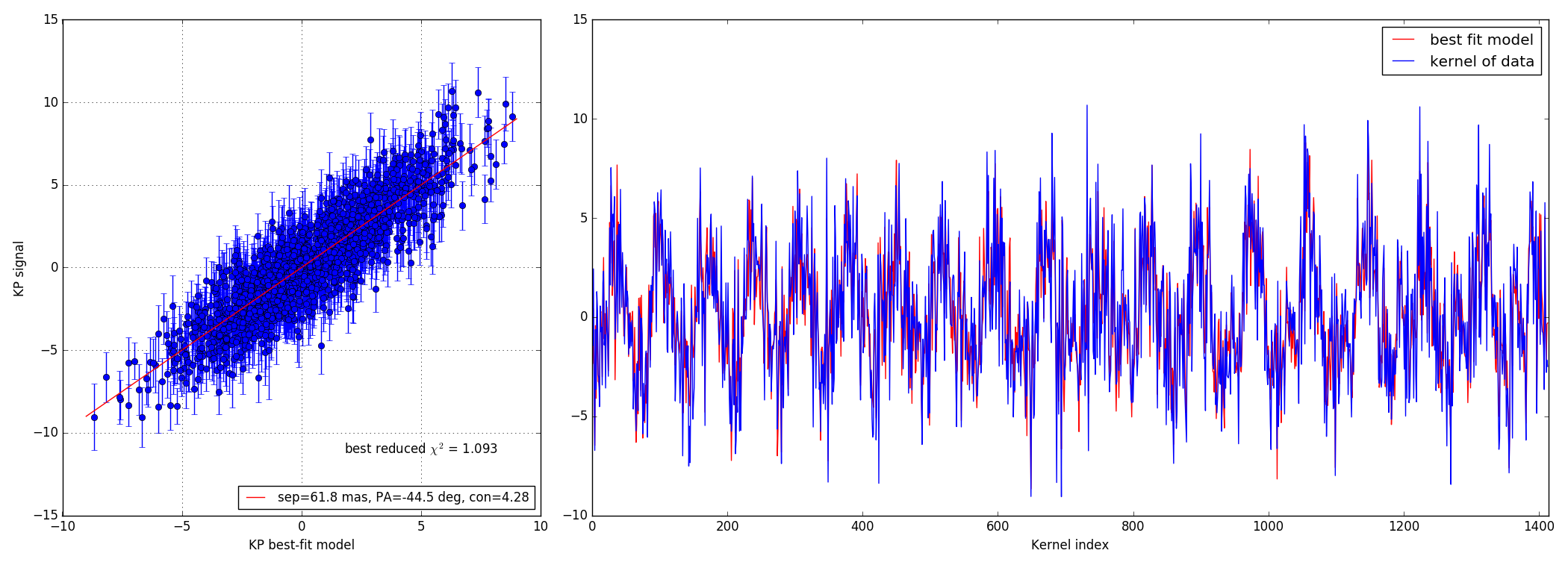
#!/usr/bin/env python

import numpy as np
import matplotlib.pyplot as plt
import matplotlib.cm as cm
import xara

plt.ion()
plt.show()

cal0  = xara.KPO(fname="jwst_model_0.15.txt")#, bfilter=0.8)
calib = cal0.copy()
trgt1 = cal0.copy()

sdir = "./bright/F480M/"
sep  = 147.0 # 73.5 #
pa   = 45.0
con  = 0.01

suffix = "CLEARP_F480M_opd_req_bb250K__00.fits"
rname  = "binary_s%.1f_p%.1f_cr%.2f__PSF_15ov_%s" % (sep, pa, con, suffix)

calib.extract_KPD(sdir+"c_"+rname, target="PSF")
trgt1.extract_KPD(sdir+"t_"+rname, target="PSF")

nobs      = np.shape(calib.KPDT)[1]
kp_model  = trgt1.kpd_binary_model([sep, -pa, 1./con], index=0, obs="KERNEL")[0]
kp_signal = np.mean(trgt1.KPDT[0], axis=0) - np.mean(calib.KPDT[0], axis=0)
kp_error  = np.sqrt(np.var(trgt1.KPDT[0],axis=0)+np.var(calib.KPDT[0], axis=0))
kp_error /= np.sqrt(nobs)

error     = kp_signal - kp_model
chi2r     = (error**2 / kp_error**2).sum() / kp_signal.size

print("----------------------------")
print("error = %9.2f mrad"  % (error.std() * 1e3, ))
print("uncrt = %9.2f mrad"  % (kp_error.std() * 1e3, ))
print("signl = %9.2f mrad"  % (kp_signal.std() * 1e3, ))
print("model = %9.2f mrad"  % (kp_model.std() * 1e3, ))
print("calib = %9.2f mrad"  % (calib.KPDT[0][0].std() * 1e3, ))
print("----------------------------")
print("reduced xi^2 = %.3f" % (chi2r, ))

# =================================================================
# =================================================================

# build a 2D map from a grid of positions specified by a size (gsz)
# and a step size (gstep) showing where the binary model best
# matches the signal recorded

gsz   = 40   # grid size
gstep = 25.0 # grid step size in mas

crit = calib.kpd_binary_match_map(gsz, gstep, kp_signal)
mmax = gstep * gsz / 2

plt.figure(2)
plt.clf()
plt.imshow(crit.reshape(gsz, gsz), extent=(-mmax, mmax, -mmax, mmax))

# =================================================================
# =================================================================
from xara.fitting import binary_KPD_fit as mfit

soluce = mfit([70.0, -45, 100.0], calib, kp_signal, kp_error)

kp_bfit = calib.kpd_binary_model(soluce[0], 0)[0]

fx, (ax1, ax2) = plt.subplots(1, 2, gridspec_kw = {'width_ratios':[1, 2]})
fx.set_size_inches(21.0, 8.0, forward=True)

ax2.plot(kp_bfit, 'r', label="best fit model")
ax2.plot(kp_signal, 'b', label="kernel of data")
ax2.set_xlabel("Kernel index")
ax2.set_xlim(0, calib.kpi.nbkp)
ax2.legend()

# ===========================================================================
# ===========================================================================

ax1.errorbar(kp_bfit, kp_signal, kp_error, marker="o", lw=0, elinewidth=1)
mmax = np.abs(kp_model).max()
bfit_lbl = "sep=%.1f mas, PA=%.1f deg, con=%.2f" % (soluce[0][0], soluce[0][1], soluce[0][2])
ax1.plot([-mmax, mmax], [-mmax, mmax], 'r', label=bfit_lbl)

ax1.set_xlabel("KP best-fit model")
ax1.set_ylabel("KP signal")
ax1.legend(loc=4, fontsize=12)
xt = ax1.get_xlim()[1] * 0.5
yt = ax1.get_ylim()[0] * 0.75
ax1.text(xt, yt, "best reduced $\chi^2$ = %.3f" % (chi2r,),
                 ha="center", fontsize=12)
fx.set_tight_layout(True)
ax1.grid()
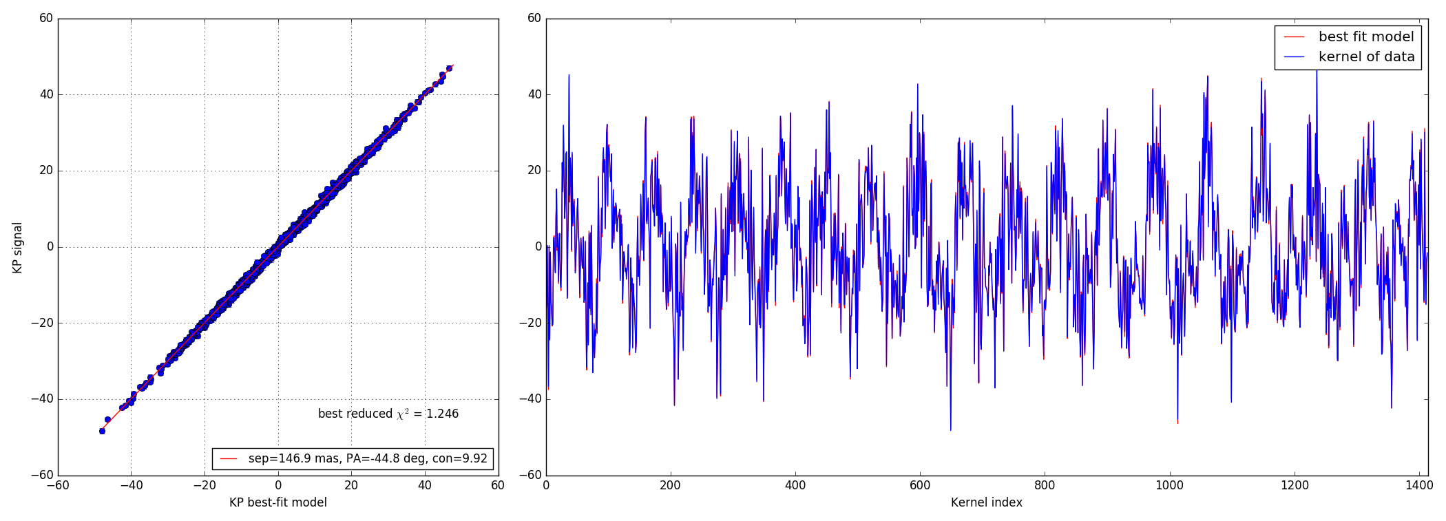
4.2 10:1 contrast ratio - 147 mas
Bright data-set
Faint data-set
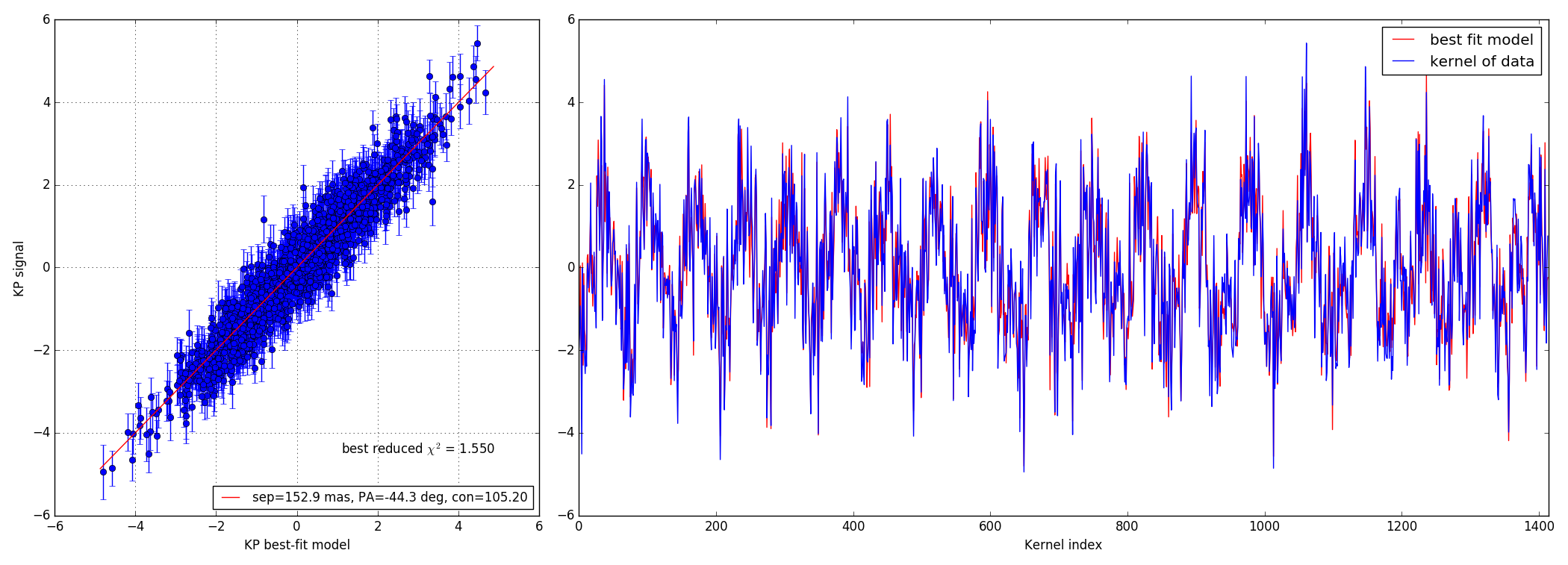
4.3 100:1 contrast ratio - 147 mas
Bright data-set
Faint data-set
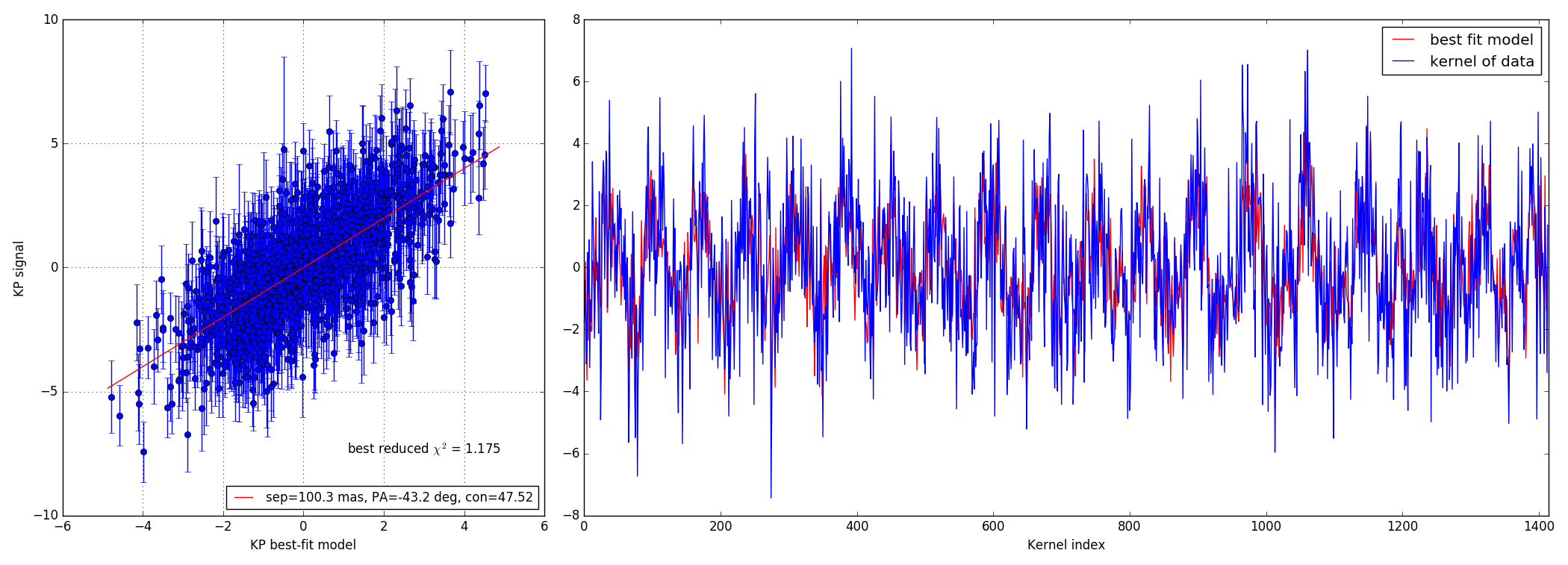
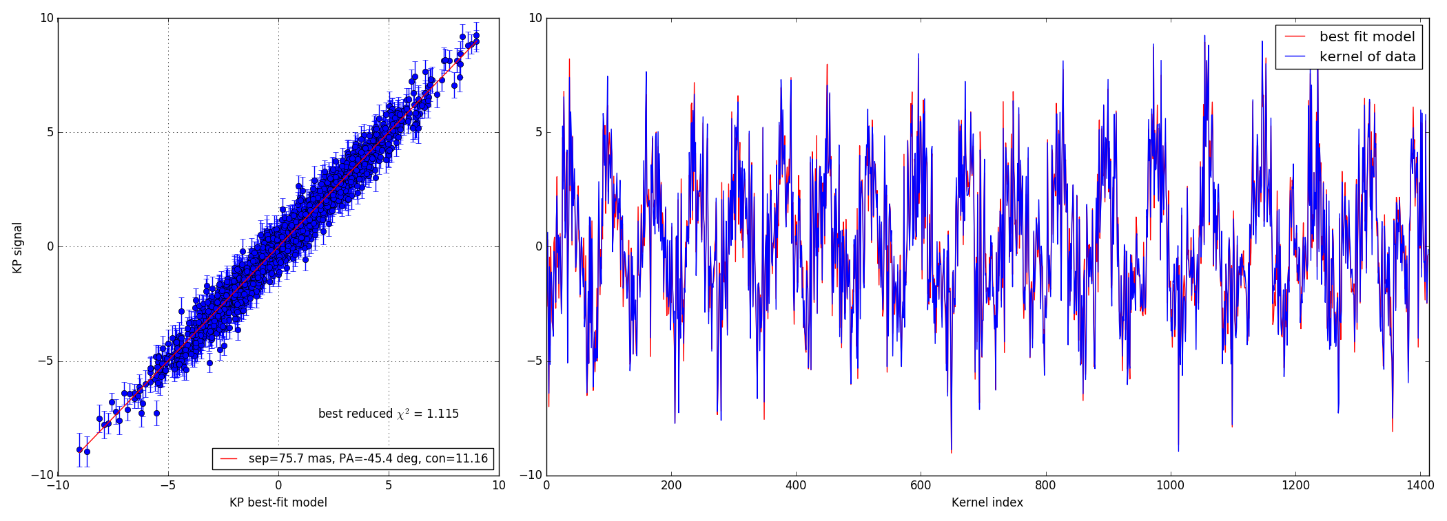
4.4 10:1 contrast ratio - 73.5 mas
Bright data-set
Faint data-set
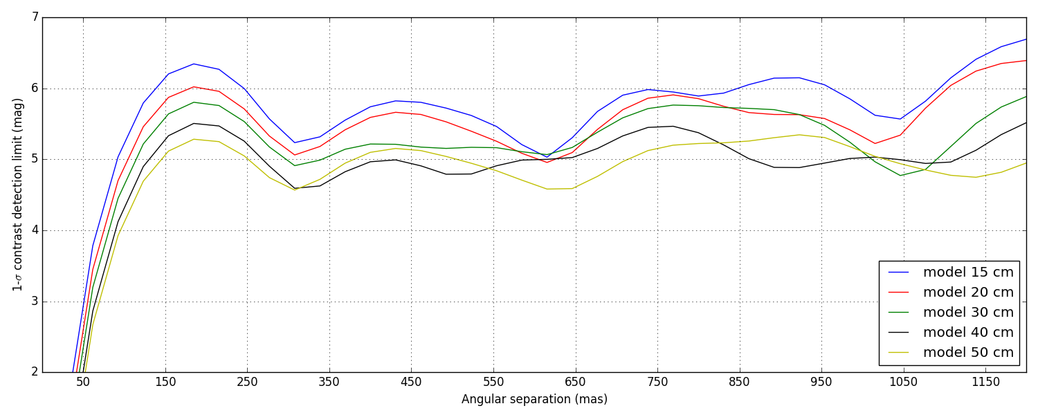
5 Contrast detection limits
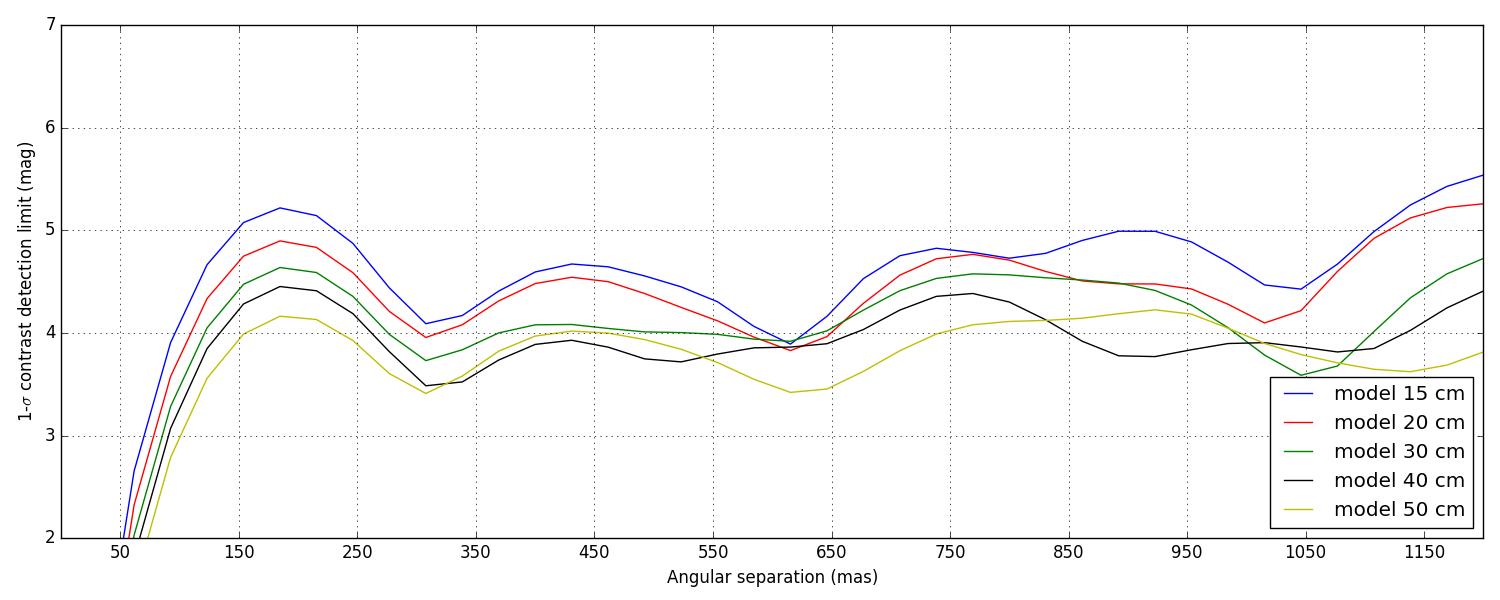
Again, these are not the final contrast curves! These contrast curves are computed using a conservative approach that does not try to take advantage of noise decorrelation techniques (see Ireland, 2013) that require the synthesis of a covariance matrix. Eventually, the analysis will.
Since here the noise is dominated by photon noise, I am looking into ways to synthetise this covariance matrix using some clever physics modeling, instead of relying on dumb force MC simulations.
Two types of data-sets were provided: bright and faint (see the introduction). The difference of illumination (from 1.2 × 10⁷ to 4 × 10⁶ photons) between the two scenarii corresponds to a \(\Delta M\) = 1.2. This difference directly reflects in the difference between the two sets of curves plotted below, the faint set being almost exactly 1.2 magnitudes lower than the bright one.
5.1 Bright data-set
5.2 Faint data-set