Fourier Eigen-Phase Wavefront Sensing
Table of Contents
1 The idea
The development of the Fourier-phase framework and XARA software was primarily driven by the astrophysics and the software is therefore fairly kernel-phase centric yet using the same framework, information of a metrologic nature can be recovered in the space orthogonal to the kernel of the phase transfer matrix. One practical consequence of this was the development of the asymmetric pupil wavefront sensor on SCExAO, for in the presence of an asymmetric aperture, it is possible to go from an image back to a wavefront. While higher level operational software was developed for SCExAO, this page attempts to explain how one can use XARA to develop one's own wavefront sensing application.
1.1 Simulation setup
This demonstration will rely on data produced by the XAOSIM simulation package also developed and maintained in the context of the KERNEL project.
import xaosim as xs

# load the SCExAO preset of XAOSIM
csz    = 300   # resolution of the simulation
APA    = 180.0 # asymmetric arm position angle (in degrees)
scexao = xs.instrument('SCExAO', csz=csz)

# change the pupil of the simulation
scexao.cam.pupil = xs.pupil.subaru_asym(
        csz, csz, csz//2,
        spiders=True, PA=APA, thick=0.15)

# visualize the pupil and the associated image
plt.imsave("scexao_asymmetric_pupil.png", scexao.cam.pupil)
plt.imsave("scexao_asymmetric_psf.png", scexao.snap()[:,32:288]**0.2)
Which produces the following images:

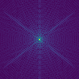
This simulation setup is fairly representative of the images produced by the IR camera inside SCExAO (aka chuckcam). The asymmetric arm introduces the additional diffraction spike along the vertical axis of the image.
1.2 Fourier-phase model creation
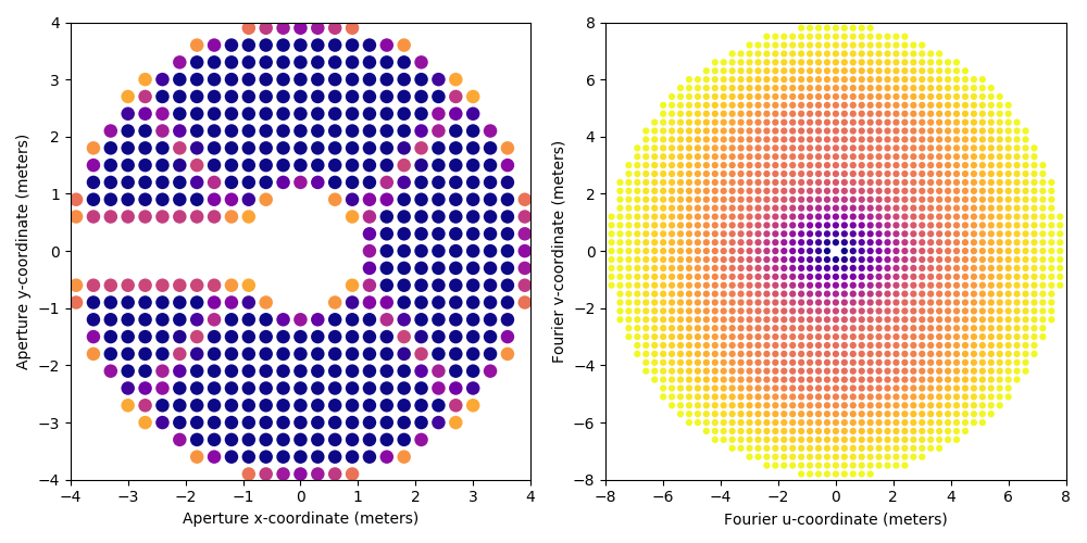
The creation of a model for wavefront sensing follows the same rules and constraints that of a model for kernel-phase analysis. We need an image featuring an oversampled representation of the pupil along with the value of the pixel scale of that representation.
#!/usr/bin/env python
import xara
import xaosim as xs

# build an oversampled image of the pupil to create the discrete model
PSZ    = 792   # Pupil pixel size
pdiam  = 7.92  # actual telescope pupil size (in meters)
APA    = 180.0 # asymmetric arm position angle (in degrees)

pup    = xs.pupil.subaru_asym(PSZ, PSZ, PSZ/2, spiders=True, PA=APA, thick=0.15)
pscale = pdiam / PSZ
model  = xara.core.create_discrete_model(pup, pscale, 0.3, binary=False, tmin=0.1)

# create the KPI data structure and save it as a multi-extension fits file
kpi = xara.KPI(array=model, bmax=7.8)#92)
kpi.save_to_file("scexao_asym.fits.gz")
1.3 Invert the phase transfer matrix
Solving the wavefront sensing requires to invert the Fourier-phase transfer matrix, which is where subtleties come into play. The asymmetry in the aperture ensures that this matrix has enough non-zero singular values to result in a full pseudo-inverse. In practice, in closed-loop, one will filter out some of the lowest singular values to improve the stability of the system. To build this pseudo-inverse, one relies on the tools shipped with the numpy.linalg package.
The following example shows how using the SVD, one would go about building a pseudo-inverse keeping 200 out of the 509 total number of available singular values.
#!/usr/bin/env python
import numpy as np

# compute the SVD of the Fourier phase transfer matrix
U, S, Vt = np.linalg.svd(kpi.TFM, full_matrices=0)

# filter some of the low singular values
neig = 200 # nomber of singular values to keep (max=509)
Sinv = 1 / S
Sinv[neig:] = 0.0

# computation of the pseudo inverse
pinv = Vt.T.dot(np.diag(Sinv)).dot(U.T)
2 Application
Equivalent to the number of actuators of a deformable mirror, the number of virtual sub-apertures across a pupil diameter imposes the size of the region surrounding a star's PSF that is used for wavefront sening purposes. The model constructed above features 26 virtual sub-apertures across a pupil diameter: the effective diameter of the control region is thus of 26 \(\lambda/D\).
To convert this into a number of pixels, one must know the plate scale of the image (16.7 mas / pixel in this simulation) and the wavelength (\(\lambda = 1.6\,\mu m\)). The size of the useful field is thus \(n = 206.265 \times 1.6 / 7.92 / 16.7 \times 26\) = 65 pixels. The original image will typically be much larger than this (if it is smaller, it means you are using a model that is not appropriate) so it is advised to crop the image down to that size. This has a dual impact:
- it reduces the size of the problem: the size of the discrete Fourier transform matrices is smaller and the computation is faster
- it reduces the impact of readout and dark current noises
In the following code snippet, an unaberrated image will be cropped, and the Fourier-phase will be extracted. This initial extraction call is the longest as the DFT matrix has to be computed first. The result of this computation is appended to the KPO data-structure for subsequent extractions (but not saved), assuming that the basic properties of the images (size, wavelength and plate-scale) remain the same: any change to these properties will require the computation of a new DFT matrix.
#!/usr/bin/env python
import xaosim as xs
import xara

# load the SCExAO preset of XAOSIM if not already running

try:
        dummy = scexao.name
except:
        csz    = 300   # computation size for the simulation
        APA    = 180.0 # asymmetric arm position angle (in degrees)
        scexao = xs.instrument('SCExAO', csz=csz)

        # change the pupil of the simulation
        scexao.cam.pupil = xs.pupil.subaru_asym(
                csz, csz, csz//2,
                spiders=True, PA=APA, thick=0.15)

# simulate an image with a static aberration
from xaosim.wavefront import sin_map
from xaosim.zernike import mkzer1
import time

sim_mode = "zernike" # anything else for sine/cosine
#sim_mode = "cos"

a0 = 0.05 # amplitude of the aberration (in radians)
z0 = 8 # zernike index (for a zernike aberration)
nc = 3 # number of cycles across the aperture (for a sine/cosine)

if "zer" in sim_mode.lower():
        scexao.atmo.set_qstatic(qstatic=a0 * mkzer1(z0, csz, csz//2, limit=True))
else:
        scexao.atmo.set_qstatic(qstatic=a0 * sin_map(csz, nc, 0, phi=np.pi/2))

ISZ = 65 # crop size of the images in pixels
img = scexao.snap()[96:96+ISZ,128:128+ISZ]

#plt.imshow(img**0.2)

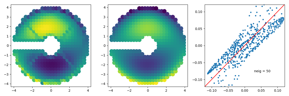
# analysis final setup
# --------------------

kpo    = xara.KPO(fname="scexao_asym.fits.gz") # load the KPO structure
U, S, Vt = np.linalg.svd(kpo.kpi.TFM, full_matrices=0)
ISZ    = 65                 # image size
pscale = scexao.cam.pscale # image plate scale in mas/pixel
cwavel = scexao.cam.wl     # central wavelength

m2pix  = xara.core.mas2rad(pscale) * ISZ / cwavel # scaling parameter

# filter some of the low singular values
neig = 200 # nomber of singular values to keep (max=509 for this model)
Sinv = 1 / S
Sinv[neig:] = 0.0

# computation of the pseudo inverse
pinv = Vt.T.dot(np.diag(Sinv)).dot(U.T)

# wavefront extraction
# --------------------
kpo.extract_KPD_single_frame(img, pscale, cwavel, recenter=True)
wft  = -pinv.dot(np.angle(kpo.CVIS[0][0]))     # compute a wavefront

# draw a picture
# --------------
from xaosim.zernike import mkzer1_vector
from xaosim.wavefront import mksin_vector

if "zer" in sim_mode.lower():
        theo = a0 * mkzer1_vector(z0, kpo.kpi.VAC)
else:
        theo = a0 * mksin_vector(kpo.kpi.VAC, nc, 0, phi=np.pi/2)

wmax = (np.abs(theo)).max()

f1 = plt.figure(figsize=(12,4))
f1.clf()
ax1 = f1.add_subplot(131)
ax1.scatter(kpo.kpi.VAC[:,0], kpo.kpi.VAC[:,1], c=np.append(0, wft),
                        vmin=-wmax, vmax=wmax, s=140)

ax2 = f1.add_subplot(132)
ax2.scatter(kpo.kpi.VAC[:,0], kpo.kpi.VAC[:,1], c=theo,
                        vmin=-wmax, vmax=wmax, s=140)

ax3 = f1.add_subplot(133)
ax3.plot(wft, theo[1:], '.')
ax3.plot([-wmax, wmax], [-wmax, wmax], 'r')
ax3.axis([-wmax,wmax,-wmax, wmax])
ax3.text(0.65*wmax, -0.65*wmax, "neig = %d" % (neig,), ha="right")
f1.set_tight_layout(True)

f1.savefig("recon_zer%d_neig%d.png" % (z0, neig,))
3 Closing the simulation
Given the semi real-time nature of the simulation by XAOSIM, it is important to properly close the simulation before eventually closing yout python shell so that garbage collection can occur and the application you are using to run your simulation does not break/crash anything. The solution is at least to ensure that the different servers that run the simulation are stopped. The icing on the cake would be to actually close the instrument object.
scexao.stop()
scexao.close()
That's all you need to remember for a graceful ending to your XAOSIM session.